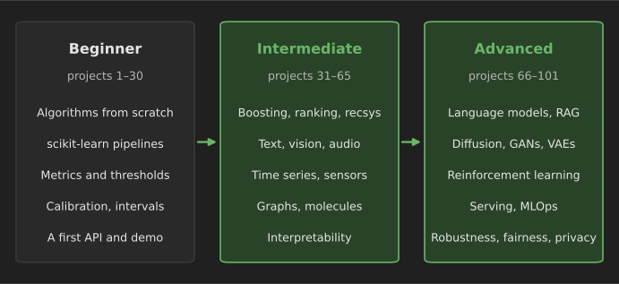
101 Machine Learning Projects, Beginner to Advanced

You learn machine learning by building models that have to work on data they have not seen. Tutorials teach the syntax, but projects teach the judgment: choosing a metric, finding leakage, deciding when a model is good enough, and explaining why it fails. This list gives you 101 machine learning projects in three levels, each written as a short brief:

Build: what you will make.
Data: a public dataset you can download, or a note when you collect your own.
Approach: the models and techniques to try, simplest first.
Evaluate: the metric, the validation scheme and the baseline you must beat.
Done when: a concrete finish line, so the project ends instead of drifting.
Stretch: an extension that turns practice into something worth showing.

How this differs from our data science project list. 101 Python data science projects focuses on asking questions of data: cleaning, exploring, visualizing and explaining. This list focuses on machine learning engineering: implementing algorithms, training and evaluating models properly, and taking them toward production. The two overlap in places, and the classic datasets used heavily there (Titanic, Iris, Palmer penguins, IMDb reviews and others) are mostly avoided here.

About the datasets. Every dataset is linked to its provider or an official mirror, and each was publicly listed when we checked in October 2026. Some require a free account or acceptance of terms, a few require a short application, and several contain personal data, so read the license and terms before you publish results or derived data. 100 machine learning datasets describes many of them in more detail, including known problems.

How to choose your next project

Pick projects by the skill you want to build next, not by how impressive the title sounds. A finished project on a modest dataset, with an honest evaluation and a clear write-up, is worth more than an abandoned attempt at something enormous.

Roadmap of the 101 projects in three levels. Beginner projects 1 to 30 cover algorithms from scratch, the scikit-learn workflow, evaluation and simple deployment. Intermediate projects 31 to 65 cover boosting and ranking, text, vision, audio, time series, recommendation, graphs and interpretability. Advanced projects 66 to 101 cover language models, generative models, reinforcement learning, production systems and trustworthy machine learning. — The three levels and the skills each one builds. Within a level, projects can be done in any order.

A practical rule from experienced practitioners is to scope the first version of any project so it can be finished in a weekend: one dataset, one baseline, one improved model and a one-page write-up. Then iterate. Community discussions about portfolios, such as threads on r/MachineLearning and r/learnmachinelearning, repeatedly mention the same complaints about beginner projects: copied tutorials, test-set leakage and accuracy reported on imbalanced data. Those are individual opinions rather than measured facts, but they match the evaluation mistakes covered at the end of this article.

The workflow every project follows

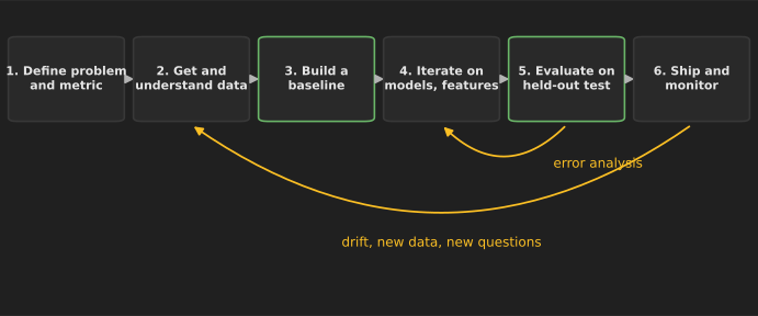
A loop of six stages: define the problem and metric, get and understand the data, build a baseline, iterate on models and features, evaluate on a held-out test set, then ship and monitor. Arrows from evaluation and monitoring lead back to the data and modeling stages, showing that the process repeats. — Most of the learning happens in the loop between evaluation and the data. The test set is used once, at the end of each iteration you plan to report.

Define the problem and the metric. Write one sentence: "Predict X for Y so that Z." Then choose the metric that matches Z: recall at a fixed false-positive rate for screening, mean absolute error in real units for forecasting, NDCG for ranking.
Understand the data. Look at the rows, the label distribution, missing values, duplicates and how the data was collected. Decide how to split: random, grouped by user or patient, or by time.
Build a baseline. Predict the majority class, the mean, "same as last week" or a simple rule. Every later model must beat it.
Iterate. Try a simple model, then a stronger one. Change one thing at a time and keep a log of what you tried.
Evaluate once on the test set. Report the test score with an estimate of its uncertainty, plus an error analysis: which cases fail and why.
Ship and monitor. Even for a portfolio project, a small API or demo and a plan for monitoring show you understand the full life cycle.

A starter template you can reuse

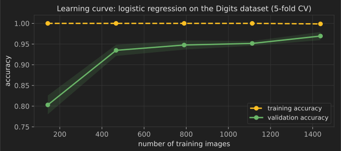
This template runs offline with a dataset bundled with scikit-learn. It compares a baseline with two models using cross-validation inside a pipeline, then checks whether more data would help with a learning curve. It was run with scikit-learn 1.9.0 on Python 3.13; the text block shows its output.

import numpy as np
from sklearn.datasets import load_digits
from sklearn.dummy import DummyClassifier
from sklearn.ensemble import HistGradientBoostingClassifier
from sklearn.linear_model import LogisticRegression
from sklearn.model_selection import StratifiedKFold, cross_val_score, learning_curve
from sklearn.pipeline import make_pipeline
from sklearn.preprocessing import StandardScaler

X, y = load_digits(return_X_y=True)
cv = StratifiedKFold(n_splits=5, shuffle=True, random_state=0)
models = {
    "baseline (most frequent)": DummyClassifier(strategy="most_frequent"),
    "logistic regression": make_pipeline(StandardScaler(), LogisticRegression(max_iter=2000)),
    "gradient boosting": HistGradientBoostingClassifier(random_state=0),
}
for name, model in models.items():
    scores = cross_val_score(model, X, y, cv=cv, scoring="accuracy")
    print(f"{name:25s} accuracy {scores.mean():.3f} ± {scores.std():.3f}")

sizes, train_scores, val_scores = learning_curve(
    models["logistic regression"], X, y, cv=cv, train_sizes=np.linspace(0.1, 1.0, 5))
for n, tr, va in zip(sizes, train_scores.mean(1), val_scores.mean(1)):
    print(f"train size {n:4d}: train {tr:.3f}  validation {va:.3f}")

baseline (most frequent)  accuracy 0.101 ± 0.001
logistic regression       accuracy 0.969 ± 0.010
gradient boosting         accuracy 0.973 ± 0.006
train size  143: train 1.000  validation 0.803
train size  467: train 1.000  validation 0.935
train size  790: train 1.000  validation 0.948
train size 1113: train 1.000  validation 0.952
train size 1437: train 0.999  validation 0.969

Learning curve for logistic regression on the Digits dataset. Training accuracy stays at about 1.00 for every training size. Validation accuracy rises from 0.80 with 143 training images to 0.97 with 1,437 images, and the gap between the two curves is still narrowing at the largest size. — A learning curve tells you what to do next. Here the validation score is still climbing and the gap to the training score is still closing, so more data would probably help. Two low curves that have met would instead suggest a more flexible model. Shaded bands show one standard deviation across the five folds.

Beginner projects (1–30)

These projects need Python, NumPy, pandas and scikit-learn, plus basic statistics. The first eight build intuition by implementing algorithms yourself; the rest practice the standard workflow on varied data. Useful background: 100 machine learning algorithms explained and 100 Python machine learning examples.

1. Linear regression from scratch with gradient descent

Build: a linear regression trained with batch gradient descent in NumPy only.
Data: the Diabetes dataset bundled with scikit-learn (load_diabetes).
Approach: standardize features, implement the mean-squared-error gradient, add an L2 penalty, and plot loss against iterations for several learning rates.
Evaluate: compare coefficients and test $R^2$ with sklearn.linear_model.Ridge at the same penalty.
Done when: your coefficients match scikit-learn's to three decimal places.
Stretch: add mini-batch SGD and momentum, and show how each changes convergence.

2. Logistic regression from scratch

Build: a binary logistic regression with the sigmoid, log loss and its gradient written by hand.
Data: Breast Cancer Wisconsin (bundled with scikit-learn as load_breast_cancer).
Approach: gradient descent first, then Newton's method; check your gradient numerically with finite differences.
Evaluate: log loss and ROC AUC on a stratified test split, against scikit-learn's LogisticRegression.
Done when: your predicted probabilities agree with scikit-learn's to within 0.01 on every test row.
Stretch: extend it to multinomial (softmax) regression on the Digits dataset.

3. Vectorized k-nearest neighbors

Build: a k-NN classifier that computes all test-to-train distances with matrix operations instead of loops.
Data: Wine (bundled with scikit-learn as load_wine).
Approach: use the identity $\|a - b\|^2 = \|a\|^2 + \|b\|^2 - 2a^\top b$ ; compare scaled and unscaled features.
Evaluate: cross-validated accuracy for $k$ from 1 to 25, and running time against a loop version.
Done when: predictions match KNeighborsClassifier exactly and you can explain why scaling changes the result.
Stretch: add a k-d tree or use FAISS and measure the speed-up on 100,000 synthetic points.

4. Decision tree from scratch

Build: a CART classifier with Gini impurity, maximum depth and minimum leaf size.
Data: UCI Car Evaluation, a small dataset of categorical car attributes.
Approach: recursive splitting; handle categorical features by one-hot encoding or by testing subsets.
Evaluate: cross-validated accuracy against DecisionTreeClassifier at the same depth.
Done when: your tree prints as readable rules and scores within one percentage point of scikit-learn's.
Stretch: turn it into a random forest with bootstrap sampling and random feature subsets.

5. k-means from scratch and image color quantization

Build: k-means with k-means++ initialization, used to reduce a photo to $k$ colors.
Data: a photo of your own, or sklearn.datasets.load_sample_image("china.jpg").
Approach: treat each pixel as a 3-D point; run k-means on a sample of pixels; recolor the image with the nearest center.
Evaluate: within-cluster sum of squares against KMeans, and file size and visual quality for $k$ = 4, 16 and 64.
Done when: your inertia is within 1% of scikit-learn's with the same initialization.
Stretch: compare with mini-batch k-means on a 12-megapixel image.

6. Naive Bayes language identifier

Build: a classifier that tells which language a sentence is written in, from character n-grams.
Data: sentences in many languages from Tatoeba (CC BY 2.0 FR).
Approach: multinomial naive Bayes on character 1- to 3-grams, written from scratch with Laplace smoothing, then compared with scikit-learn.
Evaluate: macro-averaged F1 on a held-out set with balanced languages; study the confusion between related languages such as Spanish and Portuguese.
Done when: the confusion matrix shows which language pairs are hard and your write-up explains why.
Stretch: measure accuracy against sentence length; short sentences are where the model fails.

7. The bias–variance experiment

Build: a simulation that shows underfitting and overfitting with numbers rather than words.
Data: synthetic: sample 30 noisy points from a known curve, many times.
Approach: fit polynomials of degree 1 to 15 on each sample; estimate squared bias, variance and noise at fixed test points.
Evaluate: plot the three components against degree; confirm they add up to the test error.
Done when: your plot shows the U-shaped test error and you can point to the degree with the lowest error.
Stretch: repeat with ridge regularization and show how the penalty shifts the curve.

8. Catch data leakage in cross-validation

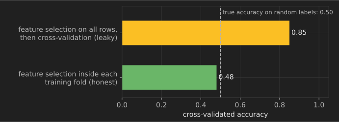
Build: a demonstration that selecting features before cross-validation produces impressive scores on pure noise.
Data: synthetic random features with random labels, so the true accuracy is 50%.
Approach: pick the 20 features most correlated with the label using all rows, then cross-validate a classifier on them; then repeat with the selection inside a Pipeline.
Evaluate: compare the two cross-validated accuracies.
Done when: you can show the leaky score and explain exactly which information leaked. The code below does this.
Stretch: find a similar leak in a published notebook or your own past work and fix it.

import numpy as np
from sklearn.feature_selection import SelectKBest, f_classif
from sklearn.linear_model import LogisticRegression
from sklearn.model_selection import cross_val_score
from sklearn.pipeline import make_pipeline

rng = np.random.default_rng(0)
X = rng.normal(size=(100, 5000))           # 5,000 features of pure noise
y = rng.integers(0, 2, size=100)            # random labels: nothing to learn

X_selected = SelectKBest(f_classif, k=20).fit_transform(X, y)   # leak: selection saw every row
leaky = cross_val_score(LogisticRegression(max_iter=1000), X_selected, y, cv=5).mean()
honest = cross_val_score(make_pipeline(SelectKBest(f_classif, k=20), LogisticRegression(max_iter=1000)), X, y, cv=5).mean()
print(f"selection outside CV: {leaky:.2f} | selection inside CV: {honest:.2f} | truth: 0.50")

selection outside CV: 0.85 | selection inside CV: 0.48 | truth: 0.50

Project 8: the same model on the same random data. Only the place where feature selection happens differs.

9. California housing with error analysis by region

Build: a house-value regression model, then a map of where it fails.
Data: California Housing, 20,640 census block groups from the 1990 census, via sklearn.datasets.fetch_california_housing (Pace and Barry, 1997).
Approach: linear regression, then gradient boosting; add latitude–longitude features such as distance to the coast.
Evaluate: mean absolute error in dollars against predicting the median value; note that the target is capped at $500,000.
Done when: you have a map of residuals and an explanation of the regions where errors are largest.
Stretch: use a spatially grouped split (hold out whole areas) and compare the error with a random split.

10. Abalone age from physical measurements

Build: a model that estimates an abalone's age from shell and weight measurements instead of counting rings under a microscope.
Data: UCI Abalone, 4,177 samples.
Approach: treat it as regression and as classification into age bands; compare linear models, random forests and boosting.
Evaluate: mean absolute error in rings against predicting the mean.
Done when: you can say whether the cheaper measurements are accurate enough to replace ring counting for a given tolerance.
Stretch: add prediction intervals with quantile regression or conformal prediction.

11. Concrete compressive strength

Build: a model predicting concrete strength from its mix ingredients and age.
Data: UCI Concrete Compressive Strength, 1,030 lab samples (Yeh, 1998).
Approach: start with linear regression on ratios (water-to-cement), then gradient boosting with monotonic constraints on age.
Evaluate: RMSE in megapascals with repeated cross-validation, because the dataset is small.
Done when: partial-dependence plots show sensible relationships, such as strength rising with age.
Stretch: fit a symbolic or small polynomial model and compare its readability with the boosted model.

12. Building heating and cooling loads

Build: a model predicting a building's heating and cooling loads from its shape.
Data: UCI Energy Efficiency, 768 simulated buildings (Tsanas and Xifara, 2012).
Approach: multi-output regression; compare one model per target with one model for both.
Evaluate: mean absolute error per target against a mean baseline.
Done when: you can rank the design features by their effect on energy use.
Stretch: note that the data comes from simulation, and discuss what that means for real buildings.

13. Handwritten letter recognition

Build: a classifier for 26 handwritten letters.
Data: EMNIST Letters, an extension of MNIST to letters.
Approach: logistic regression and random forest on pixels, then a small CNN.
Evaluate: accuracy and the most confused letter pairs (for example, "l" and "i").
Done when: you have a confusion analysis with example images for the top five confusions.
Stretch: combine with EMNIST Digits and handle the ambiguity between "O" and "0".

14. Dry bean variety classification

Build: a classifier for seven bean varieties from shape features extracted from images.
Data: UCI Dry Bean, 13,611 beans (Koklu and Ozkan, 2020).
Approach: scaling plus logistic regression, SVM and gradient boosting; examine correlated shape features.
Evaluate: macro F1, since classes are imbalanced.
Done when: you have identified which varieties are confused and which features would separate them.
Stretch: reduce to the five most useful features and measure what accuracy you lose.

15. Banknote authentication with a readable model

Build: a forged-banknote detector that a bank clerk could follow as rules.
Data: UCI Banknote Authentication, 1,372 images summarized by four wavelet features.
Approach: a depth-limited decision tree and logistic regression; compare with an SVM.
Evaluate: accuracy is very high on this dataset, so focus on the false-negative rate and on how simple the model can be.
Done when: a tree of depth 3 or less is documented as rules, with its error rate.
Stretch: explain why near-perfect scores on a small dataset may not carry over to new printers or scanners.

16. Choose a decision threshold for a screening model

Build: a classifier plus a documented choice of threshold for a screening use case.
Data: Breast Cancer Wisconsin (bundled with scikit-learn).
Approach: fit a calibrated model; plot precision, recall and false-positive rate against the threshold; use TunedThresholdClassifierCV for a target metric.
Evaluate: recall at a fixed false-positive rate, with confidence intervals from bootstrapping the test set.
Done when: you recommend a threshold, state its expected recall and false-positive rate, and explain the trade-off in plain language.
Stretch: add a cost matrix and choose the threshold that minimizes expected cost.

17. Probability calibration

Build: a study of how well different models' predicted probabilities match reality.
Data: UCI Adult (Census Income), 48,842 people from the 1994 U.S. census.
Approach: compare logistic regression, random forest, gradient boosting and naive Bayes; calibrate with Platt scaling and isotonic regression.
Evaluate: reliability diagrams, Brier score and log loss on a held-out set.
Done when: you can show which models are over- or under-confident and how calibration changes that.
Stretch: check calibration separately by sex and race, and discuss what differences would mean for a real decision.

18. Bankruptcy prediction with imbalanced classes

Build: a model that predicts which companies go bankrupt, where bankruptcies are rare.
Data: UCI Polish Companies Bankruptcy, financial ratios for Polish companies over five years (Zięba, Tomczak and Tomczak, 2016).
Approach: gradient boosting with class weights; compare with resampling; handle many missing ratios.
Evaluate: precision–recall AUC and recall at a fixed precision, not accuracy.
Done when: you can show why accuracy is misleading here and which metric you used instead.
Stretch: train on early years and test on a later year to see how much performance drops.

19. Movie genre from plot summaries

Build: a multi-label classifier that tags a film's genres from its plot.
Data: the CMU Movie Summary Corpus, 42,306 plot summaries from Wikipedia with metadata from Freebase.
Approach: TF-IDF with one-vs-rest logistic regression, then sentence embeddings with a linear classifier.
Evaluate: micro and macro F1 over the 20 most common genres; per-genre precision and recall.
Done when: you have a table of which genres are predictable from text and which are not.
Stretch: tune a separate threshold for each genre to maximize F1.

20. Grid search versus random search versus successive halving

Build: an experiment comparing hyperparameter search strategies under a fixed time budget.
Data: Covertype, 581,012 forest plots, via sklearn.datasets.fetch_covtype (also at UCI).
Approach: tune HistGradientBoostingClassifier with GridSearchCV, RandomizedSearchCV and HalvingRandomSearchCV.
Evaluate: best validation accuracy reached against wall-clock time for each strategy.
Done when: you have a chart of accuracy against time for the three strategies and a recommendation.
Stretch: add Bayesian optimization with Optuna and repeat with several random seeds.

21. Feature importance that does not mislead

Build: a comparison of feature-importance methods, including their failure modes.
Data: UCI Auto MPG, fuel economy of 398 cars from the 1970s and early 1980s.
Approach: compare linear coefficients, impurity-based importance, permutation importance and SHAP values; add a random noise column and a duplicated feature.
Evaluate: where does the noise column rank? How is importance split between the duplicates?
Done when: you can explain, with your own results, why impurity importance can mislead.
Stretch: read the scikit-learn guide on permutation importance and reproduce its warning about correlated features.

22. A pipeline for messy tabular data

Build: one Pipeline with a ColumnTransformer that imputes, encodes, scales and models a real messy dataset.
Data: Hotel booking demand, about 119,000 bookings from two Portuguese hotels (Antonio, de Almeida and Nunes, 2019).
Approach: predict cancellations; remove columns that leak the outcome (such as the reservation status); handle dates and high-cardinality countries.
Evaluate: ROC AUC with a time-based split by arrival date.
Done when: the pipeline runs end to end from raw CSV to predictions, and you list every leaky column you removed and why.
Stretch: compare a random split with the time split and explain the difference.

23. Prediction intervals for power plant output

Build: a model that predicts electrical output with a range, not just a point.
Data: UCI Combined Cycle Power Plant, 9,568 hourly readings (Tüfekci, 2014).
Approach: gradient boosting with quantile loss for the 5th and 95th percentiles; compare with split conformal prediction.
Evaluate: interval coverage (target 90%) and average width on a held-out set.
Done when: your intervals reach their target coverage on test data and you report their width.
Stretch: check whether coverage holds separately for hot and cold conditions.

24. Serve a model with a small API

Build: a REST endpoint that loads a trained model and returns predictions.
Data: any model from projects 9–23.
Approach: save the full pipeline with joblib or skops, serve it with FastAPI, validate inputs with Pydantic, and package it in a container.
Evaluate: a test that sends a request and checks the response; latency over 1,000 requests.
Done when: someone else can run one command and get a prediction from curl.
Stretch: add input validation that rejects out-of-range values and log every prediction.

25. A draw-a-digit web demo

Build: a web page where users draw a digit and see the model's prediction and confidence.
Data: the Digits dataset (bundled with scikit-learn) or MNIST.
Approach: train a small CNN; preprocess the drawing to match the training images (size, centering, stroke width); deploy with Gradio or Streamlit.
Evaluate: collect 50 drawings from friends and measure accuracy on them, not just on the test set.
Done when: the demo works for people who did not build it, and you report the gap between test accuracy and real-drawing accuracy.
Stretch: add a "wrong?" button that saves corrected examples for retraining.

26. Wholesale customer segments

Build: a customer segmentation with clusters that a sales team could use.
Data: UCI Wholesale Customers, annual spending of 440 clients of a Portuguese distributor.
Approach: log-transform spending, then compare k-means, Gaussian mixtures and hierarchical clustering.
Evaluate: silhouette scores, cluster stability under resampling, and whether each cluster has a clear description.
Done when: each segment has a name, a profile and a suggested action.
Stretch: check the stability of your clusters by refitting on bootstrap samples and measuring agreement.

27. Eigenfaces

Build: a face-recognition pipeline using PCA features, to understand what PCA captures.
Data: Labeled Faces in the Wild via sklearn.datasets.fetch_lfw_people (also in TensorFlow Datasets).
Approach: PCA to 150 components, then an SVM; visualize the top eigenfaces.
Evaluate: per-person precision and recall; accuracy against the number of components.
Done when: you can show what the first components encode (lighting, pose) and how many you need.
Stretch: read about the limits of LFW (mostly well-known public figures, unbalanced demographics) and discuss them.

28. Benchmark anomaly detectors

Build: a fair comparison of anomaly detection methods on several labeled datasets.
Data: small benchmark datasets from ODDS, where anomalies are labeled.
Approach: isolation forest, local outlier factor, one-class SVM and robust covariance, trained without labels.
Evaluate: ROC AUC and precision at the true number of anomalies, using labels only for evaluation.
Done when: you have a results table across at least five datasets and a note on which method wins where.
Stretch: add a simple autoencoder and see whether it beats the classical methods.

29. Sunspot forecasting

Build: a monthly forecast of sunspot numbers.
Data: the monthly mean total sunspot number from SILSO, Royal Observatory of Belgium, from 1749.
Approach: naive and seasonal-naive baselines, exponential smoothing, ARIMA, then gradient boosting on lag features.
Evaluate: rolling-origin evaluation with mean absolute error 12 months ahead.
Done when: you have a backtest table showing whether any model beats the baselines.
Stretch: compare your forecast of the current solar cycle with the official forecasts published by NOAA's Space Weather Prediction Center.

30. Write a model card for one of your models

Build: a model card documenting the purpose, data, metrics, limitations and ethical considerations of a model you trained.
Data: any model from this section.
Approach: follow the structure proposed in "Model Cards for Model Reporting" (Mitchell et al., 2019).
Evaluate: ask someone unfamiliar with the project whether the card tells them when not to use the model.
Done when: the card includes performance broken down by at least one relevant subgroup.
Stretch: add a datasheet for the training data (Gebru et al., 2021).

Intermediate projects (31–65)

These projects add larger data, unstructured inputs (text, images, audio, graphs), time series and more careful evaluation. You will need PyTorch or a similar framework for some of them, and a GPU helps for the vision and audio projects (free cloud notebooks are enough).

31. Gradient boosting on 11 million rows

Build: a classifier that separates a particle-physics signal from background.
Data: UCI HIGGS, 11 million simulated collision events (Baldi, Sadowski and Whiteson, 2014).
Approach: histogram gradient boosting or LightGBM; compare the 21 low-level features with the 7 high-level physics features.
Evaluate: ROC AUC on the official last 500,000 rows used as the test set.
Done when: you report AUC against training-set size (100,000, 1 million, 10 million rows) and training time.
Stretch: train an MLP and compare it with boosting as the data grows.

32. Encoding high-cardinality categories

Build: a comparison of categorical encodings on data that is almost entirely IDs.
Data: Amazon.com Employee Access Challenge on Kaggle (free account).
Approach: one-hot encoding with logistic regression, target encoding with cross-fitting (sklearn.preprocessing.TargetEncoder), and CatBoost.
Evaluate: ROC AUC with stratified cross-validation; check for target leakage in naive target encoding.
Done when: you can show the score inflation caused by naive target encoding and the fix.
Stretch: add pairwise combinations of categories as new features.

33. Click-through rate prediction with feature hashing

Build: a CTR model that trains on data too large for one-hot encoding in memory.
Data: Avazu Click-Through Rate Prediction on Kaggle, about 40 million ad impressions.
Approach: feature hashing with online logistic regression (SGDClassifier.partial_fit), then a factorization machine or a small deep model.
Evaluate: log loss on the last day, trained on earlier days.
Done when: your model trains in streaming fashion with bounded memory and beats predicting the average CTR.
Stretch: measure calibration, since ad auctions use the probability directly.

34. Learning to rank for web search

Build: a ranking model that orders documents for a query.
Data: Microsoft Learning to Rank (MSLR-WEB10K), 10,000 queries with relevance labels.
Approach: pointwise regression, then LambdaMART with LightGBM's lambdarank objective.
Evaluate: NDCG@10 on the provided test fold.
Done when: LambdaMART beats the pointwise baseline and you can explain why ranking objectives help.
Stretch: compute per-query NDCG and study the queries where the model fails.

35. Next-item recommendation

Build: a model that predicts the next product a user will review.
Data: Amazon Reviews 2023, more than 570 million reviews across 33 categories; start with one small category.
Approach: popularity and item-to-item co-occurrence baselines, then a sequential model such as GRU4Rec or SASRec.
Evaluate: Recall@10 and NDCG@10 with a leave-last-out split per user, ordered by time.
Done when: your sequential model beats the popularity baseline on a time-respecting split.
Stretch: report results separately for users with short and long histories.

36. A two-tower retrieval model

Build: a recommender that embeds users and items separately so candidates can be retrieved with nearest-neighbor search.
Data: MovieLens 32M, 32 million ratings (redistribution not permitted).
Approach: matrix factorization with ALS as a baseline, then a two-tower network with in-batch negatives; index items with FAISS.
Evaluate: Recall@100 on held-out later ratings, and query latency.
Done when: retrieval of the top 100 items takes milliseconds and recall beats the ALS baseline.
Stretch: add item features (genres, tags) and test cold-start items.

37. Star ratings from review text

Build: a model that predicts a review's 1–5 star rating from its text.
Data: the Yelp Open Dataset (requires accepting Yelp's terms).
Approach: TF-IDF with ordinal or multinomial logistic regression, then a fine-tuned small transformer.
Evaluate: mean absolute error in stars and macro F1; inspect 3-star reviews.
Done when: your error analysis explains which reviews are inherently ambiguous.
Stretch: treat it as regression and compare with classification.

38. Named-entity recognition in another language

Build: a tagger that finds person, organization and location names in a language other than English.
Data: WikiANN, entity annotations derived from Wikipedia in many languages.
Approach: a conditional random field on word features, then a fine-tuned multilingual transformer such as XLM-RoBERTa.
Evaluate: entity-level F1 with seqeval, not token accuracy.
Done when: you report F1 per entity type and examples of errors.
Stretch: train on one language and test zero-shot on a related one.

39. Toxic comment classification

Build: a multi-label classifier for several types of toxic comments.
Data: the Jigsaw Toxic Comment Classification Challenge on Kaggle. The comments contain offensive language.
Approach: TF-IDF with logistic regression per label, then a fine-tuned transformer.
Evaluate: mean column-wise ROC AUC, plus a check of false positives on comments that mention identity groups without being toxic.
Done when: you report both overall AUC and the identity-term false-positive check.
Stretch: read the follow-up Jigsaw competition on unintended bias and apply its bias metrics.

40. Claim verification against Wikipedia

Build: a system that labels a claim as supported, refuted or not enough information, with evidence sentences.
Data: FEVER, 185,445 claims written from Wikipedia (Thorne et al., 2018).
Approach: retrieve candidate sentences with BM25, then classify claim–evidence pairs with a fine-tuned natural-language-inference model.
Evaluate: label accuracy and the FEVER score, which also requires correct evidence.
Done when: you show how much retrieval errors limit final accuracy.
Stretch: test whether the model relies on words in the claim alone by training a claim-only baseline.

41. A small translation model

Build: a sequence-to-sequence translator for short image captions.
Data: Multi30k, about 30,000 English–German caption pairs.
Approach: an LSTM encoder–decoder with attention, then a small transformer; tokenize with byte-pair encoding.
Evaluate: BLEU or chrF with sacrebleu on the official test set.
Done when: the transformer beats the LSTM and you show example translations with typical errors.
Stretch: compare greedy decoding with beam search.

42. Spoken digit recognition

Build: a classifier for spoken digits 0–9.
Data: the Free Spoken Digit Dataset, short recordings from several speakers.
Approach: MFCC features with an SVM, then a CNN on log-mel spectrograms.
Evaluate: accuracy with a speaker-independent split (test speakers never seen in training).
Done when: you report the gap between random and speaker-independent splits.
Stretch: record your own voice and test on it.

43. Music genre classification and its pitfalls

Build: a genre classifier, then an investigation of whether its score means anything.
Data: GTZAN (Kaggle mirror), 1,000 30-second clips in 10 genres.
Approach: a CNN on spectrograms; then read Sturm's analysis of the dataset's repetitions, mislabelings and distortions (Sturm, 2013).
Evaluate: accuracy with an artist-filtered split versus a random split.
Done when: you show how much accuracy drops when the same artist cannot appear in both training and test data.
Stretch: repeat on the larger, better-documented FMA dataset.

44. Street View house numbers

Build: a CNN that reads digits cropped from Google Street View photos.
Data: SVHN, over 600,000 digit images (Netzer et al., 2011).
Approach: a small CNN trained from scratch, with and without data augmentation and batch normalization.
Evaluate: test accuracy and an ablation table of what each change contributes.
Done when: you have an ablation table with at least three runs per configuration.
Stretch: use the "extra" training images and measure the gain from more data.

45. Flower recognition with transfer learning

Build: a fine-grained image classifier for 102 flower species from a pretrained network.
Data: Oxford 102 Flowers.
Approach: linear probe on frozen features, then full fine-tuning of a pretrained ResNet or ViT.
Evaluate: top-1 accuracy on the official test split; accuracy against the number of training images per class.
Done when: you show how many labeled images per class you need for a given accuracy.
Stretch: compare with zero-shot classification using a CLIP model.

46. Pedestrian detection

Build: an object detector that draws boxes around pedestrians.
Data: the Penn-Fudan Database for Pedestrian Detection and Segmentation, 170 images.
Approach: fine-tune a pretrained Faster R-CNN from torchvision; this dataset is used in PyTorch's own detection tutorial.
Evaluate: mean average precision at IoU 0.5 and 0.5–0.95.
Done when: you report mAP and show failure cases (occlusion, small people).
Stretch: add the masks and train Mask R-CNN for instance segmentation.

47. Pet segmentation with a U-Net

Build: a model that separates pets from the background pixel by pixel.
Data: Oxford-IIIT Pet, 37 breeds with pixel-level trimaps.
Approach: a U-Net trained from scratch, then one with a pretrained encoder.
Evaluate: intersection over union (IoU) and Dice score on the test split.
Done when: the pretrained-encoder version beats the scratch version and you show boundary errors.
Stretch: measure IoU separately for cats and dogs and for small and large animals.

48. Exercise repetition counter from video

Build: an app that counts squats or push-ups from webcam video.
Data: your own recorded videos (record with consent if other people appear).
Approach: a pretrained pose-estimation model (such as MediaPipe Pose) to get joint positions, then a rule or a small classifier on joint angles over time.
Evaluate: count error against manual counts on 20 videos you did not use for tuning.
Done when: the counter is within one repetition on most test videos.
Stretch: add form feedback, such as flagging squats that are not deep enough.

49. Handwritten text recognition

Build: a model that transcribes lines of handwritten English.
Data: the IAM Handwriting Database (free registration).
Approach: a CNN–LSTM with CTC loss, then a pretrained transformer OCR model such as TrOCR.
Evaluate: character error rate and word error rate on writers not seen in training.
Done when: you report CER with a writer-independent split.
Stretch: add a language model to correct likely spelling errors.

50. One forecasting model for 370 electricity customers

Build: a global model that forecasts many related time series at once.
Data: UCI Electricity Load Diagrams 2011–2014, 15-minute consumption of 370 customers in Portugal.
Approach: seasonal-naive baseline, one model per series, then one gradient-boosting model across all series with lag and calendar features.
Evaluate: mean absolute scaled error over a rolling backtest, 24 hours ahead.
Done when: you show whether the global model beats per-series models.
Stretch: forecast quantiles and evaluate with the pinball loss.

51. Weather forecasting with neural networks

Build: a 24-hour temperature forecast from past weather readings.
Data: the Max Planck Institute for Biogeochemistry weather station data, Jena, recorded every 10 minutes.
Approach: persistence and seasonal baselines, gradient boosting on lags, then an LSTM and a temporal convolutional network.
Evaluate: mean absolute error on the final year, trained on earlier years.
Done when: you show whether the neural models beat boosting, with the same inputs.
Stretch: add a multi-horizon forecast and plot error against horizon.

52. Anomaly detection in streaming metrics

Build: a detector that flags anomalies in server and sensor metrics as data streams in.
Data: the Numenta Anomaly Benchmark (NAB), 58 labeled time series (Lavin and Ahmad, 2015).
Approach: rolling z-scores, seasonal decomposition residuals, then isolation forest on windowed features.
Evaluate: NAB's scoring, which rewards early detection, plus precision and recall within labeled windows.
Done when: your detector runs one point at a time and beats a static threshold.
Stretch: read critiques of time-series anomaly benchmarks (Wu and Keogh, 2021) and test whether simple baselines score suspiciously well.

53. Bearing fault diagnosis from vibration

Build: a classifier that identifies bearing faults from vibration signals.
Data: the Case Western Reserve University Bearing Data Center.
Approach: frequency-domain features with gradient boosting, then a 1-D CNN on raw signal windows.
Evaluate: accuracy when training on some motor loads and testing on another, not just on random windows.
Done when: you show the gap between random-window and load-shift splits, which is the realistic one.
Stretch: discuss why overlapping windows in both training and test sets inflate scores.

54. Human activity recognition from phone sensors

Build: a classifier for walking, sitting, standing and other activities from smartphone accelerometer and gyroscope data.
Data: UCI Human Activity Recognition Using Smartphones, 30 volunteers.
Approach: the provided handcrafted features with boosting, then a 1-D CNN on the raw signals.
Evaluate: accuracy with the official subject-wise split.
Done when: you report per-activity results and explain the sitting–standing confusion.
Stretch: collect your own phone data and test the model on it.

55. Deep learning versus boosted trees on tabular data

Build: a fair benchmark of an MLP, a tabular transformer and gradient boosting.
Data: the OpenML-CC18 benchmark suite of classification tasks (Bischl et al., 2021).
Approach: equal tuning budgets for each model family; repeat across many datasets.
Evaluate: average rank across datasets, with the number of datasets where each model wins.
Done when: your conclusion is stated with the tuning budget and the datasets it applies to.
Stretch: compare your results with the published findings of Grinsztajn et al. (2022).

56. Explaining a credit model

Build: a credit-risk classifier with global and individual explanations.
Data: Statlog (German Credit Data), 1,000 loan applicants with a published cost matrix.
Approach: logistic regression and gradient boosting; SHAP values for explanations; the dataset's cost matrix for threshold choice.
Evaluate: expected cost using the published cost matrix, not accuracy.
Done when: you produce a plain-language explanation for three individual decisions and check them for plausibility.
Stretch: generate counterfactual explanations ("what would need to change for approval?") and check that they are actionable.

57. Survival analysis for patient outcomes

Build: a model of time until recurrence that handles patients whose outcome is not yet known (censoring).
Data: the German Breast Cancer Study Group 2 data, available in scikit-survival as load_gbsg2.
Approach: Kaplan–Meier curves, a Cox proportional-hazards model, then a random survival forest.
Evaluate: the concordance index and time-dependent Brier score.
Done when: you explain why dropping censored patients or treating them as "no event" biases results.
Stretch: check the proportional-hazards assumption and discuss what to do when it fails.

58. Active learning to save labeling effort

Build: a loop where the model chooses which examples a human should label next.
Data: 20 Newsgroups via sklearn.datasets.fetch_20newsgroups; simulate the human by revealing labels on request.
Approach: start with 20 labels; compare random sampling, uncertainty sampling and diversity-based sampling.
Evaluate: accuracy against the number of labels used, averaged over several runs.
Done when: you show how many labels uncertainty sampling saves to reach a target accuracy.
Stretch: add a cold-start strategy based on clustering the unlabeled data.

59. Semi-supervised image classification

Build: an image classifier trained with few labels and many unlabeled images.
Data: STL-10, with 5,000 labeled and 100,000 unlabeled images.
Approach: supervised baseline on labels only, then pseudo-labeling and a FixMatch-style consistency method (Sohn et al., 2020).
Evaluate: test accuracy with 250, 1,000 and 5,000 labels.
Done when: you show the gain from unlabeled data at each label budget.
Stretch: check whether pseudo-labels are biased toward easy classes.

60. Hyperparameter optimization for a neural network

Build: an automated tuning study for a small image classifier.
Data: Fashion-MNIST, 70,000 clothing images.
Approach: Optuna with the tree-structured Parzen estimator and pruning of unpromising trials; tune learning rate, width, dropout and batch size.
Evaluate: validation accuracy against trial count; final test accuracy of the best configuration.
Done when: you report which hyperparameters mattered most (Optuna's importance plot) and the variance across seeds.
Stretch: compare with random search at the same budget.

61. Knowledge distillation for text classification

Build: a small, fast sentiment model that learns from a larger one.
Data: SST-2 from the GLUE benchmark (Wang et al., 2018).
Approach: fine-tune a base-size transformer as teacher, then train a small student on the teacher's soft labels (Hinton, Vinyals and Dean, 2015).
Evaluate: accuracy against latency and model size for teacher, student trained alone and distilled student.
Done when: the distilled student beats the student trained on hard labels alone.
Stretch: distill into a non-transformer model such as a BiLSTM or a linear model on embeddings.

62. Node classification on a citation network

Build: a graph neural network that predicts a paper's topic from its text features and citations.
Data: Cora, 2,708 papers and 5,429 citation links (Sen et al., 2008), available in PyTorch Geometric as Planetoid.
Approach: logistic regression on features only, label propagation on the graph only, then a GCN using both.
Evaluate: accuracy on the standard split, averaged over random seeds.
Done when: you show that combining features and graph structure beats either alone.
Stretch: try a graph attention network and visualize the learned attention weights.

63. Link prediction for collaborations

Build: a model that predicts which researchers will collaborate in the future.
Data: ogbl-collab from the Open Graph Benchmark, a co-authorship graph split by year.
Approach: heuristics such as common neighbors and Adamic–Adar, then a GNN-based link predictor.
Evaluate: Hits@50 with OGB's official evaluator and time-based split.
Done when: you report whether the GNN beats the heuristics, which is not guaranteed.
Stretch: analyze errors by node degree.

64. Molecular solubility prediction

Build: a model that predicts how well a molecule dissolves in water from its structure.
Data: the ESOL (Delaney) dataset from MoleculeNet (Wu et al., 2018), about 1,100 molecules.
Approach: RDKit fingerprints with random forests, then a message-passing neural network on molecular graphs.
Evaluate: RMSE with a scaffold split, which keeps similar molecules out of the test set.
Done when: you report both random-split and scaffold-split RMSE and explain the gap.
Stretch: add uncertainty estimates and check whether high uncertainty predicts high error.

65. Land-cover classification from satellite images

Build: a classifier for ten land-cover types from Sentinel-2 satellite image patches.
Data: EuroSAT, 27,000 labeled patches (Helber et al., 2019).
Approach: random forest on band statistics, then a CNN on RGB, then a CNN on all 13 spectral bands.
Evaluate: accuracy with a geographically separated split, in addition to the random split.
Done when: you show how much the extra spectral bands help.
Stretch: apply the model to a new Sentinel-2 scene of your region from the Copernicus Data Space.

Advanced projects (66–101)

These projects involve training neural networks from scratch, large language models, generative models, reinforcement learning, production systems and trustworthy machine learning. Most need a GPU; cloud notebooks are enough for the smaller ones if you keep models small.

66. A tiny autograd engine

Build: a scalar automatic-differentiation engine and a small neural network library on top of it.
Data: synthetic two-moons data from scikit-learn.
Approach: implement a Value class that records operations and runs backpropagation through the graph, as in Andrej Karpathy's micrograd.
Evaluate: compare every gradient with PyTorch's on random expressions.
Done when: your gradients match PyTorch's to within $10^{-6}$ and an MLP trained with your engine separates the moons.
Stretch: vectorize it to work on tensors.

67. A character-level GPT from scratch

Build: a small decoder-only transformer that generates text one character at a time.
Data: Tiny Shakespeare, about 1 MB of Shakespeare's plays.
Approach: implement causal self-attention, positional embeddings and the training loop; compare with nanoGPT for reference.
Evaluate: validation loss (bits per character) against model size and context length.
Done when: your model's validation loss beats a bigram baseline and its samples have recognizable structure.
Stretch: add a byte-pair-encoding tokenizer and compare.

68. Train and analyze a BPE tokenizer

Build: a byte-pair-encoding tokenizer trained from scratch, and an analysis of how it splits text.
Data: WikiText-103, about 100 million tokens from Wikipedia articles.
Approach: implement BPE merges yourself on a sample, then train a full tokenizer with Hugging Face tokenizers.
Evaluate: tokens per word for English, code and another language at vocabulary sizes of 8,000, 32,000 and 64,000.
Done when: you show how vocabulary size changes sequence length and which languages pay a "token tax".
Stretch: measure how numbers are split and discuss the effect on arithmetic.

69. Instruction-tune a small open model

Build: a small open language model fine-tuned to follow instructions in a specific domain.
Data: databricks-dolly-15k, 15,000 human-written instruction–response pairs (CC BY-SA 3.0).
Approach: supervised fine-tuning with LoRA adapters on a model with roughly 1 billion parameters.
Evaluate: side-by-side human ratings of base versus tuned responses on 50 held-out prompts, plus an automated benchmark.
Done when: you report the win rate of the tuned model, judged blind.
Stretch: check whether the tuned model got worse on a general benchmark (catastrophic forgetting).

70. Evaluate a retrieval-augmented generation pipeline

Build: a question-answering system that retrieves documents and generates answers, plus the evaluation to measure it.
Data: a dataset from the BEIR benchmark (Thakur et al., 2021), such as SciFact or FiQA.
Approach: BM25, dense retrieval and a hybrid of both; generate answers with a small open model.
Evaluate: retrieval Recall@k and nDCG@10 separately from answer quality; check whether answers are supported by retrieved text.
Done when: you can show how much retrieval quality limits answer quality.
Stretch: add a reranker and measure its effect on cost and quality.

71. Fine-tune an embedding model for search

Build: a sentence-embedding model adapted to a search task.
Data: MS MARCO passage ranking, real Bing queries with relevant passages.
Approach: start from a pretrained embedding model; fine-tune with contrastive loss and hard negatives mined with BM25.
Evaluate: MRR@10 on the development set before and after fine-tuning.
Done when: fine-tuning improves MRR and you test the model on a BEIR dataset to check generalization.
Stretch: compress the embeddings (lower dimension or 8-bit) and measure the quality loss.

72. A careful language-model evaluation

Build: an evaluation harness for grade-school math problems that measures accuracy reliably.
Data: GSM8K, 8,500 math word problems (Cobbe et al., 2021).
Approach: prompt several open models with and without step-by-step reasoning; extract the final answer with strict parsing.
Evaluate: exact-match accuracy with confidence intervals; rerun with different sampling seeds.
Done when: you report accuracy with uncertainty and show how much it changes with prompt wording.
Stretch: test for contamination by rewording problems and changing their numbers.

73. Preference tuning with DPO

Build: a small language model tuned to prefer helpful, harmless responses, using direct preference optimization.
Data: Anthropic HH-RLHF, human preference comparisons between pairs of responses. It includes harmful content by design.
Approach: supervised fine-tuning, then DPO (Rafailov et al., 2023) on the preference pairs.
Evaluate: win rate against the SFT model on held-out prompts, judged by humans or a separate judge model, plus a check for length bias.
Done when: you report win rate and average response length, and discuss whether length explains the gain.
Stretch: compare DPO with PPO-based RLHF on the same budget.

74. Vision transformer versus ResNet on small data

Build: a comparison of a vision transformer and a ResNet trained from scratch.
Data: CIFAR-10, 60,000 small images in 10 classes.
Approach: implement patch embedding and a small ViT; train both models with the same budget and augmentation.
Evaluate: test accuracy against training set size (10%, 50% and 100%).
Done when: you show where the ViT catches up, if it does, and relate it to the original ViT paper's discussion of data scale (Dosovitskiy et al., 2020).
Stretch: visualize attention maps for a few images.

75. Self-supervised contrastive learning

Build: an image encoder trained without labels, then evaluated with a linear classifier.
Data: STL-10's 100,000 unlabeled images, with its labeled split for evaluation.
Approach: implement SimCLR (Chen et al., 2020): two augmentations per image and a contrastive loss.
Evaluate: linear-probe accuracy, against a supervised baseline trained on the 5,000 labels.
Done when: you report linear-probe accuracy against batch size and augmentation strength.
Stretch: try a non-contrastive method such as BYOL or SimSiam.

76. Zero-shot image search with CLIP

Build: a text-to-image search engine over your own photo collection.
Data: your photos, plus COCO captions for evaluation.
Approach: embed images and text with a pretrained CLIP model (Radford et al., 2021) from OpenCLIP; index with FAISS.
Evaluate: Recall@5 for text-to-image retrieval on COCO's 5,000-image validation set.
Done when: search works on your own photos and you report COCO recall.
Stretch: probe for biased associations by searching for occupations and inspecting the results.

77. A diffusion model from scratch

Build: a denoising diffusion model that generates small images.
Data: Fashion-MNIST or CIFAR-10.
Approach: implement DDPM (Ho, Jain and Abbeel, 2020) with a small U-Net and a linear or cosine noise schedule.
Evaluate: visual samples plus Fréchet Inception Distance (FID) against the test set.
Done when: samples are recognizable and you report FID against the number of sampling steps.
Stretch: add classifier-free guidance to generate a chosen class.

78. Variational autoencoder latent space

Build: a VAE whose latent space you can explore and interpolate in.
Data: Fashion-MNIST.
Approach: convolutional encoder and decoder; vary the KL weight (the β in β-VAE).
Evaluate: reconstruction error, KL divergence, and whether latent dimensions capture separate attributes.
Done when: you show smooth interpolations between items and the effect of β on reconstruction quality.
Stretch: use the VAE's reconstruction error for anomaly detection on MNIST digits.

79. A GAN and its failure modes

Build: a deep convolutional GAN, and a record of how training fails.
Data: Fashion-MNIST.
Approach: DCGAN architecture; deliberately trigger mode collapse (for example, by unbalancing learning rates) and then fix it.
Evaluate: FID and a per-class count of generated samples, using a pretrained classifier.
Done when: you document one collapse and the change that fixed it.
Stretch: add a gradient penalty (WGAN-GP) and compare stability.

80. Image super-resolution

Build: a model that upscales low-resolution images by a factor of four.
Data: DIV2K, 1,000 high-resolution images.
Approach: bicubic interpolation baseline, then a CNN trained with pixel loss, then with perceptual or adversarial loss.
Evaluate: PSNR and SSIM, plus a small blind human preference test.
Done when: you show that the model with the best PSNR is not always the one people prefer.
Stretch: test on photos from your phone, which have different noise than DIV2K's downsampled images.

81. Speech recognition for another language

Build: a speech-to-text model fine-tuned for a language with less training data than English.
Data: Mozilla Common Voice, crowd-sourced recordings in hundreds of languages.
Approach: evaluate a pretrained Whisper model zero-shot (Radford et al., 2022), then fine-tune a small version.
Evaluate: word error rate on the official test split, with speakers kept separate.
Done when: you report WER before and after fine-tuning.
Stretch: break WER down by accent or gender where the metadata allows.

82. Speaker diarization of meetings

Build: a pipeline that answers "who spoke when" in a meeting recording.
Data: the AMI Meeting Corpus, 100 hours of meeting recordings.
Approach: voice activity detection, speaker embeddings, then clustering; compare with a pretrained pipeline such as pyannote.audio.
Evaluate: diarization error rate on held-out meetings.
Done when: you report DER and analyze errors during overlapping speech.
Stretch: combine with speech recognition to produce a speaker-labeled transcript.

83. Deep Q-learning for a control task

Build: an agent that learns to land a lunar module in simulation.
Data: none; the Gymnasium LunarLander environment generates experience.
Approach: implement DQN with a replay buffer and target network, then add double DQN.
Evaluate: average return over 100 evaluation episodes, across at least five random seeds.
Done when: your agent averages above 200, the score at which the environment documentation considers it solved.
Stretch: plot learning curves across seeds and discuss the variance.

84. PPO for continuous control

Build: an agent that learns to walk or balance in a physics simulator.
Data: none; the MuJoCo environments in Gymnasium, such as HalfCheetah or Hopper.
Approach: implement PPO with generalized advantage estimation; compare with a library implementation such as Stable-Baselines3 or CleanRL.
Evaluate: average return against environment steps over several seeds.
Done when: your implementation reaches returns similar to the reference implementation with the same budget.
Stretch: run an ablation of PPO's implementation details (Huang et al., 2022).

85. Offline reinforcement learning

Build: an agent trained only from a fixed dataset of past behavior, without interacting with the environment.
Data: datasets from Minari, the Farama Foundation's standard for offline RL datasets.
Approach: behavior cloning baseline, then conservative Q-learning or implicit Q-learning.
Evaluate: normalized return in the simulator after training on the fixed data.
Done when: you show when offline RL beats behavior cloning and when it does not.
Stretch: vary the dataset quality (expert, medium, random) and plot the effect.

86. A bandit recommender simulator

Build: a simulator that tests exploration strategies for recommendations before using them on real users.
Data: MovieLens 32M, turned into a replay simulator (show an item only if the user actually rated it).
Approach: epsilon-greedy, UCB and Thompson sampling, then a contextual bandit with user features.
Evaluate: cumulative reward against rounds, with the replay method of Li et al. (2011).
Done when: you show the regret curves and explain the replay method's bias.
Stretch: add a delay between showing an item and observing the reward.

87. AlphaZero-style self-play

Build: an agent that learns Connect Four by playing against itself.
Data: none; games are generated by self-play.
Approach: Monte Carlo tree search guided by a small policy-value network, trained on its own games (Silver et al., 2018).
Evaluate: win rate against a fixed-depth minimax player and against earlier versions of itself.
Done when: the agent beats a depth-4 minimax player more than half the time.
Stretch: Connect Four is solved, so compare its moves with a perfect solver.

88. Do pretrained forecasting models beat simple baselines?

Build: an evaluation of a pretrained time-series foundation model against classical methods.
Data: the M4 competition series (Makridakis, Spiliotis and Assimakopoulos, 2020).
Approach: seasonal naive, exponential smoothing and a gradient-boosting global model, against a zero-shot pretrained forecaster such as Chronos (Ansari et al., 2024).
Evaluate: sMAPE and MASE per frequency, using M4's official horizons.
Done when: you report which frequencies the pretrained model wins and loses.
Stretch: check whether M4 series could have been part of the pretrained model's training data.

89. A tabular foundation model on small datasets

Build: a comparison of a pretrained tabular model with tuned gradient boosting on small datasets.
Data: small classification tasks from OpenML.
Approach: TabPFN (Hollmann et al., 2025) without tuning, against gradient boosting with a tuning budget.
Evaluate: ROC AUC and total compute time across at least 20 datasets.
Done when: you report where each approach wins, by dataset size and number of features.
Stretch: test the limits of dataset size the pretrained model supports.

90. Serve a model under a latency budget

Build: a prediction service that meets a 95th-percentile latency target under load.
Data: any image or text model from earlier projects.
Approach: export to ONNX, serve with ONNX Runtime behind an API, add dynamic batching, and load test with Locust or k6.
Evaluate: throughput and p50/p95/p99 latency at increasing request rates.
Done when: you show the request rate at which the p95 target breaks, and what fixed it.
Stretch: compare CPU and GPU serving costs per 1,000 predictions.

91. Quantization and pruning

Build: a smaller, faster version of a trained model with a measured accuracy cost.
Data: a fine-tuned image or text classifier from earlier projects.
Approach: post-training dynamic and static int8 quantization in PyTorch; magnitude pruning with fine-tuning.
Evaluate: accuracy, model size and latency on a CPU for each version.
Done when: you produce a table of the trade-offs and pick a version for a stated latency goal.
Stretch: try quantization-aware training and compare.

92. Shadow deployment and an online A/B test

Build: a system that runs a new model version in "shadow" mode beside the current one, then tests it on live traffic.
Data: a simulated stream from any dataset with timestamps, such as the hotel bookings in project 22.
Approach: log both models' predictions on the same requests; compare offline; then route a share of traffic to the new model and analyze the outcome.
Evaluate: agreement rate in shadow mode; a pre-registered test of the business metric with a power calculation.
Done when: you produce a decision memo that recommends shipping or not, with evidence.
Stretch: add automatic rollback if live error rates exceed a threshold.

93. Find label errors in a famous dataset

Build: a tool that flags likely mislabeled examples.
Data: CIFAR-10 or another benchmark studied in "Pervasive Label Errors in Test Sets" (Northcutt, Athalye and Mueller, 2021).
Approach: confident learning with out-of-fold predicted probabilities, using the cleanlab library.
Evaluate: manually review the top 100 flagged examples and record how many are truly wrong.
Done when: you report precision of the flags on manual review.
Stretch: retrain after removing or fixing errors and measure the effect.

94. Robustness to image corruptions

Build: an evaluation of how image classifiers degrade under noise, blur, weather and compression.
Data: CIFAR-10-C from the robustness benchmark (Hendrycks and Dietterich, 2019).
Approach: evaluate a standard model, then one trained with augmentations such as AugMix.
Evaluate: accuracy per corruption type and severity; mean corruption error.
Done when: you show which corruptions hurt most and which augmentations help.
Stretch: test on real photos with the same corruptions, such as your phone's camera in low light.

95. Adversarial examples and adversarial training

Build: attacks that fool an image classifier with imperceptible changes, and a defense.
Data: CIFAR-10.
Approach: FGSM and PGD attacks (Madry et al., 2017); adversarial training with PGD.
Evaluate: clean accuracy and accuracy under attack at several perturbation sizes.
Done when: you show the trade-off between clean and robust accuracy.
Stretch: evaluate with a stronger attack suite such as AutoAttack to check that robustness is real.

96. Skin-tone performance gaps in a dermatology model

Build: a skin-condition classifier and an audit of its accuracy across skin tones.
Data: Fitzpatrick 17k, clinical images labeled with Fitzpatrick skin type (Groh et al., 2021).
Approach: fine-tune a pretrained CNN; train on lighter skin types only, then on all types.
Evaluate: accuracy by Fitzpatrick type with confidence intervals.
Done when: you report the performance gap and how training data composition changes it.
Stretch: read the dataset's documentation on how skin type was labeled and discuss the label uncertainty. This is a research exercise, not a diagnostic tool.

97. Differential privacy and membership inference

Build: a model trained with differential privacy, and an attack that tests what a normal model leaks.
Data: UCI Adult or CIFAR-10.
Approach: a membership-inference attack (Shokri et al., 2017) on a normal model, then DP-SGD training with the Opacus library.
Evaluate: attack success (ROC AUC) and model accuracy at several privacy budgets ε.
Done when: you show the privacy–accuracy trade-off curve.
Stretch: explain in plain language what a given ε does and does not guarantee.

98. Federated learning simulation

Build: a model trained across simulated devices that never share their raw data.
Data: FEMNIST from the LEAF benchmark, handwriting split naturally by writer (Caldas et al., 2018).
Approach: federated averaging (McMahan et al., 2017) with the Flower framework; compare with centralized training.
Evaluate: accuracy against communication rounds, with different shares of clients per round.
Done when: you show the gap between federated and centralized accuracy and how non-identical client data affects it.
Stretch: add secure aggregation or differential privacy to the federated updates.

99. Test whether saliency maps are trustworthy

Build: saliency maps for an image classifier, and tests of whether they reflect the model.
Data: a fine-tuned classifier from project 45 or 47.
Approach: Grad-CAM and integrated gradients; apply the model- and data-randomization sanity checks of Adebayo et al. (2018).
Evaluate: similarity of maps before and after randomizing the model's weights.
Done when: you show which methods pass the sanity checks.
Stretch: run a deletion test: remove the most salient pixels and measure the drop in confidence.

100. A miniature scaling-law study

Build: language models of five sizes trained on the same data, and a fit of loss against size.
Data: TinyStories, short synthetic stories designed for small models (Eldan and Li, 2023).
Approach: train decoder-only transformers from about 1 million to 50 million parameters with the same token budget per parameter.
Evaluate: validation loss against parameters and compute; fit a power law.
Done when: your plot shows a clear trend and you state the fitted exponent with its uncertainty.
Stretch: compare your fit with published scaling laws (Kaplan et al., 2020; Hoffmann et al., 2022) and explain the differences.

101. Capstone: a documented ML system for a real problem

Build: an end-to-end system for a problem you or someone you know actually has.
Data: data you collect or obtain with permission, documented with a datasheet.
Approach: everything from this list that applies: baseline, careful split, model iteration, calibrated outputs, a service, monitoring.
Evaluate: the metric your user cares about, measured on data collected after you built the model.
Done when: a real user has used it, you have a model card and datasheet, and you have written a post-launch review of what broke.
Stretch: keep it running for a month and report how performance changed.

Mistakes that weaken ML projects

Leakage. The most common and most damaging error. Fit every preprocessing step inside cross-validation (project 8), split by group or time when rows are related, and remove features that would not exist at prediction time.
The wrong metric. Accuracy on imbalanced data, RMSE when the business cares about large errors only, or a metric nobody downstream uses.
No baseline. Without one, a reader cannot tell whether 85% is impressive.
Tuning on the test set. Choosing a model, threshold or feature set by looking at test scores turns the test set into a validation set. Keep a final test set you look at once.
Ignoring variance. Small datasets and neural network training produce noisy results. Report the spread across folds or seeds.
Unreproducible results. Pin library versions, fix random seeds, and make the notebook run from top to bottom.
Stopping at the score. Error analysis, a demo and a short write-up of limitations are what make a project convincing.

Where to go next

Learn how each model works in 100 machine learning algorithms explained.
Choose data with care using 100 machine learning datasets.
Get more from your features with 101 feature engineering techniques.
See how organizations apply these ideas in 100 machine learning applications across industries.
For exploration and analysis projects, see 101 Python data science projects.
Find practitioners writing about their own projects in the blog directory.

References

Kelly, M., Longjohn, R., & Nottingham, K. The UCI Machine Learning Repository. University of California, Irvine. archive.ics.uci.edu
Mitchell, M., et al. (2019). "Model Cards for Model Reporting." FAT* 2019. arxiv.org/abs/1810.03993
Gebru, T., et al. (2021). "Datasheets for Datasets." Communications of the ACM, 64(12). arxiv.org/abs/1803.09010
Kapoor, S., & Narayanan, A. (2023). "Leakage and the reproducibility crisis in machine-learning-based science." Patterns, 4(9). doi.org/10.1016/j.patter.2023.100804
Northcutt, C. G., Athalye, A., & Mueller, J. (2021). "Pervasive Label Errors in Test Sets Destabilize Machine Learning Benchmarks." NeurIPS 2021 Datasets and Benchmarks. arxiv.org/abs/2103.14749
Grinsztajn, L., Oyallon, E., & Varoquaux, G. (2022). "Why do tree-based models still outperform deep learning on typical tabular data?" arxiv.org/abs/2207.08815
Sculley, D., et al. (2015). "Hidden Technical Debt in Machine Learning Systems." NeurIPS 2015. papers.nips.cc
scikit-learn developers. "Common pitfalls and recommended practices." scikit-learn.org
Sutton, R. S., & Barto, A. G. (2018). Reinforcement Learning: An Introduction (2nd ed.). incompleteideas.net
Farama Foundation. Gymnasium documentation. gymnasium.farama.org