A machine learning algorithm is a procedure that turns data into a model: a function that makes predictions, finds structure or chooses actions. There are hundreds of them, but most practical work uses a few dozen, and those fall into a handful of families. Once you understand the family, a new algorithm is usually a variation on an idea you already know.
This guide explains 100 of the most widely used algorithms, grouped by family. Every entry answers the same five questions:
- What it is: the core idea in plain language.
- How it works: the formula or intuition behind it.
- When to use it: the problems it suits, its strengths and its limits.
- Python example: a short, runnable snippet using scikit-learn, NumPy or PyTorch.
- Real-world application: how the algorithm is used in practice, with a source where a specific deployment is named.
About the code. The snippets were run with Python 3.13, scikit-learn 1.9.0, NumPy 2.3.5, SciPy 1.18.1, pandas 3.0.3 and PyTorch 2.14 (CPU), and the text under each snippet is what it printed. Each snippet stands alone. They use datasets bundled with scikit-learn (Iris, Wine, Digits, Breast Cancer Wisconsin, Diabetes) or synthetic data, so they run offline in seconds. Scores are illustrations of what the code does, not benchmarks: an algorithm that wins on a toy dataset can lose on your data. Last digits may differ on other machines, and PyTorch results can vary slightly between versions. Three entries (XGBoost, CatBoost and UMAP) need libraries outside that list; their snippets are marked as not run, and the text says so.
Which "best"? No algorithm is best in general; the no-free-lunch results say that averaged over all possible problems, every learner performs the same (Wolpert, 1996). On real tabular data, gradient-boosted trees are a very strong default (Grinsztajn et al., 2022); on images, audio and text, deep networks dominate. The list below is ordered by family, not by rank.
If you want more end-to-end code, the companion article 100 Python machine learning examples shows complete workflows (pipelines, tuning, evaluation) for specific applications. This article focuses on how each algorithm works and when to choose it. For the math underneath, see linear algebra for machine learning, probability and statistics for data science and optimization techniques.
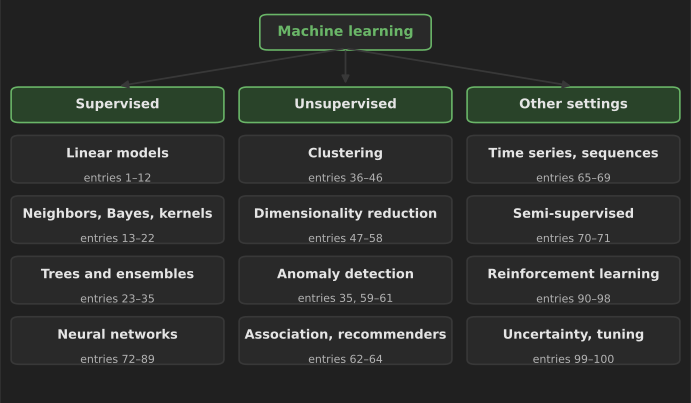
How to choose an algorithm
Before reading 100 entries, it helps to know the questions that narrow the choice:
- Do you have labels? If every example has a known answer, it is supervised learning (classification for categories, regression for numbers). Without labels, it is unsupervised (clustering, dimensionality reduction, anomaly detection). With a few labels and many unlabeled examples, consider semi-supervised methods. If the system learns by acting and receiving rewards, it is reinforcement learning.
- What kind of data? Tables of mixed numeric and categorical columns favor tree ensembles and linear models. Images, audio and raw text favor neural networks. Sequences and time series have their own methods.
- How much data? With hundreds of rows, simple models with strong assumptions (linear models, naive Bayes, small trees) often win. With millions of rows, flexible models (boosting, deep networks) can use the extra data.
- Do you need to explain the decision? Regulated decisions such as credit and medical triage often favor models whose reasoning can be inspected, such as linear models, small trees or monotonic boosted models.
- What does an error cost? This decides the metric (accuracy, recall at a fixed false-positive rate, mean absolute error), which matters more than the algorithm.
Always start with a baseline (predict the most common class or the mean) and a simple model. A complex model is only worth its cost if it beats them on held-out data.
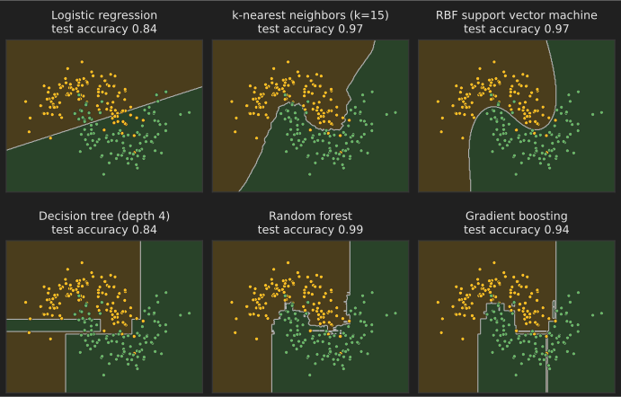
Linear and generalized linear models
Linear models predict with a weighted sum of the features. They are fast, need little data, and their weights can be read directly, which is why they remain the first model to try and the standard in regulated settings.
1. Linear regression (ordinary least squares)
What it is: fits the straight line (or flat plane) through the data that best predicts a number.
How it works: the prediction is . Ordinary least squares chooses the weights that minimize the sum of squared errors , which has the closed-form solution (computed in practice with a QR or SVD decomposition, not by inverting the matrix).
When to use it: as the first model for any numeric target, and whenever you need coefficients you can explain. It assumes the relationship is roughly linear and that errors are independent with constant variance. It is sensitive to outliers and to strongly correlated features, which make individual coefficients unstable.
from sklearn.datasets import load_diabetes
from sklearn.linear_model import LinearRegression
from sklearn.model_selection import train_test_split

X, y = load_diabetes(return_X_y=True)
X_train, X_test, y_train, y_test = train_test_split(X, y, random_state=0)
model = LinearRegression().fit(X_train, y_train)
print("R^2 on test data:", round(model.score(X_test, y_test), 3))
print("first three coefficients:", model.coef_[:3].round(1))
R^2 on test data: 0.359
first three coefficients: [ -43.3 -208.7  593.4]
Real-world application: estimating how price, promotion and season affect sales (marketing mix models), and the hedonic regression models that national statistics offices use to adjust price indexes for quality changes.
2. Ridge regression
What it is: linear regression with a penalty that keeps the weights small.
How it works: minimizes . The L2 penalty shrinks all coefficients toward zero, which reduces variance when features are correlated or numerous. The solution is , which exists even when is singular.
When to use it: whenever you would use linear regression but have many features, correlated features or few rows. Choose by cross-validation. Scale the features first, because the penalty treats all coefficients alike.
from sklearn.datasets import load_diabetes
from sklearn.linear_model import RidgeCV
from sklearn.model_selection import cross_val_score
from sklearn.pipeline import make_pipeline
from sklearn.preprocessing import StandardScaler

X, y = load_diabetes(return_X_y=True)
model = make_pipeline(StandardScaler(), RidgeCV(alphas=[0.1, 1, 10, 100]))
print("mean CV R^2:", round(cross_val_score(model, X, y, cv=5).mean(), 3))
print("chosen alpha:", model.fit(X, y)[-1].alpha_)
mean CV R^2: 0.48
chosen alpha: 1.0
Real-world application: genomic prediction in plant and animal breeding, where thousands of genetic markers predict a trait from a few hundred animals; ridge-type models (often called RR-BLUP or GBLUP) are a standard tool there (Meuwissen, Hayes and Goddard, 2001).
3. Lasso regression
What it is: linear regression that sets some weights exactly to zero, so it also selects features.
How it works: minimizes (Tibshirani, 1996). The corners of the L1 penalty make zero coefficients optimal for weak features. It is solved by coordinate descent.
When to use it: when you suspect only a few of many features matter and you want a sparse, readable model. With groups of correlated features it tends to pick one arbitrarily; elastic net (next) is more stable.
from sklearn.datasets import load_diabetes
from sklearn.linear_model import LassoCV
from sklearn.pipeline import make_pipeline
from sklearn.preprocessing import StandardScaler

X, y = load_diabetes(return_X_y=True)
model = make_pipeline(StandardScaler(), LassoCV(cv=5, random_state=0)).fit(X, y)
lasso = model[-1]
print("alpha:", round(lasso.alpha_, 3))
print("features kept:", (lasso.coef_ != 0).sum(), "of", X.shape[1])
alpha: 0.079
features kept: 9 of 10
Real-world application: selecting a small panel of biomarkers or genes from thousands of candidates in medical studies, where a short list is cheaper to measure and easier to validate.
4. Elastic net
What it is: a blend of ridge and lasso penalties.
How it works: the penalty is , where (l1_ratio) moves between ridge () and lasso () (Zou and Hastie, 2005). It keeps lasso's sparsity but shares weight across correlated features.
When to use it: high-dimensional data with correlated features, such as text n-grams or gene expression. Tune both and . The synthetic features below are uncorrelated, so cross-validation picks pure lasso (); that is a legitimate result, and on correlated data a mixed value usually wins.
from sklearn.datasets import make_regression
from sklearn.linear_model import ElasticNetCV

X, y = make_regression(n_samples=200, n_features=50, n_informative=8, noise=10, random_state=0)
model = ElasticNetCV(l1_ratio=[0.2, 0.5, 0.8, 1.0], cv=5, random_state=0).fit(X, y)
print("l1_ratio:", model.l1_ratio_, "| nonzero coefficients:", (model.coef_ != 0).sum())
l1_ratio: 1.0 | nonzero coefficients: 19
Real-world application: epigenetic "clocks" that estimate a person's biological age from DNA methylation levels at a few hundred sites were built with elastic net regression (Horvath, 2013).
5. Polynomial regression
What it is: linear regression on powers and products of the features, so a linear model can fit curves.
How it works: expand into (and interaction terms such as ), then fit ordinary or ridge regression. The model is still linear in its weights, so the same solvers apply.
When to use it: smooth, low-dimensional curved relationships. High degrees overfit and behave wildly outside the training range; splines are usually safer for flexible curves.
import numpy as np
from sklearn.linear_model import LinearRegression
from sklearn.pipeline import make_pipeline
from sklearn.preprocessing import PolynomialFeatures

rng = np.random.default_rng(0)
x = rng.uniform(-3, 3, 100).reshape(-1, 1)
y = 0.5 * x[:, 0] ** 2 - x[:, 0] + rng.normal(0, 0.5, 100)
for degree in (1, 2):
    model = make_pipeline(PolynomialFeatures(degree), LinearRegression()).fit(x, y)
    print(f"degree {degree}: R^2 = {model.score(x, y):.3f}")
degree 1: R^2 = 0.545
degree 2: R^2 = 0.954
Real-world application: calibration curves for sensors and lab instruments, where a quadratic or cubic maps a raw reading to a physical quantity.
6. Logistic regression
What it is: the standard linear model for yes/no classification. It outputs a probability.
How it works: passes the linear score through the sigmoid, , and fits the weights by maximizing the likelihood (equivalently, minimizing log loss). Each coefficient is a change in the log-odds per unit of the feature.
When to use it: any binary classification problem as a baseline, and when you need calibrated probabilities and explainable coefficients. It draws a straight decision boundary, so curved boundaries need engineered features.
from sklearn.datasets import load_breast_cancer
from sklearn.linear_model import LogisticRegression
from sklearn.model_selection import train_test_split
from sklearn.pipeline import make_pipeline
from sklearn.preprocessing import StandardScaler

X, y = load_breast_cancer(return_X_y=True)
X_train, X_test, y_train, y_test = train_test_split(X, y, stratify=y, random_state=0)
model = make_pipeline(StandardScaler(), LogisticRegression(max_iter=1000)).fit(X_train, y_train)
print("accuracy:", round(model.score(X_test, y_test), 3))
print("P(benign) for first test case:", model.predict_proba(X_test[:1])[0, 1].round(3))
accuracy: 0.958
P(benign) for first test case: 0.996
Real-world application: credit scorecards. Lenders have long built scorecards with logistic regression on binned features, because each feature's contribution to the score can be shown to regulators and explained to applicants (Siddiqi, Credit Risk Scorecards, Wiley).
7. Multinomial (softmax) regression
What it is: logistic regression for more than two classes.
How it works: computes one linear score per class and turns the scores into probabilities with the softmax . It is trained with cross-entropy loss, the same loss used in the final layer of most neural network classifiers.
When to use it: multiclass problems where you want probabilities for every class and a simple, fast model.
from sklearn.datasets import load_wine
from sklearn.linear_model import LogisticRegression
from sklearn.model_selection import cross_val_score
from sklearn.pipeline import make_pipeline
from sklearn.preprocessing import StandardScaler

X, y = load_wine(return_X_y=True)
model = make_pipeline(StandardScaler(), LogisticRegression(max_iter=1000))
print("classes:", sorted(set(y.tolist())), "| mean CV accuracy:", round(cross_val_score(model, X, y, cv=5).mean(), 3))
classes: [0, 1, 2] | mean CV accuracy: 0.983
Real-world application: routing support tickets or documents into one of several categories from bag-of-words features, where a linear softmax model on TF-IDF features is a strong, cheap baseline.
8. Poisson regression (a generalized linear model)
What it is: regression for counts, such as claims per policy or visits per day.
How it works: models the log of the expected count as linear, , and assumes a Poisson distribution for . Generalized linear models swap the distribution and link function to fit other targets: Gamma for positive amounts, Tweedie for amounts with many zeros.
When to use it: non-negative count targets, especially when exposure varies (use an offset or sample weights). Overdispersed counts may need a negative binomial model instead.
import numpy as np
from sklearn.linear_model import PoissonRegressor

rng = np.random.default_rng(0)
X = rng.normal(size=(1000, 2))
y = rng.poisson(np.exp(0.3 + 0.8 * X[:, 0] - 0.5 * X[:, 1]))
model = PoissonRegressor(alpha=1e-4).fit(X, y)
print("intercept:", round(model.intercept_, 2), "| coefficients:", model.coef_.round(2))
intercept: 0.3 | coefficients: [ 0.79 -0.51]
Real-world application: insurance pricing. Actuaries model claim frequency with Poisson GLMs and claim severity with Gamma GLMs; scikit-learn's documentation reproduces this on French motor insurance data (scikit-learn example).
9. Quantile regression
What it is: predicts a chosen percentile of the target (for example, the 90th) instead of the mean.
How it works: minimizes the pinball loss, which weights under-predictions by and over-predictions by (Koenker and Bassett, 1978). With it predicts the median.
When to use it: when the cost of error is asymmetric, or when you need prediction intervals. Fitting the 5th and 95th percentiles gives a 90% interval.
import numpy as np
from sklearn.linear_model import QuantileRegressor

rng = np.random.default_rng(0)
x = rng.uniform(0, 10, 300).reshape(-1, 1)
y = 2 * x[:, 0] + rng.normal(0, 0.5 + 0.3 * x[:, 0])  # noise grows with x
for q in (0.1, 0.5, 0.9):
    m = QuantileRegressor(quantile=q, alpha=0, solver="highs").fit(x, y)
    print(f"q={q}: prediction at x=8 is {m.predict([[8]])[0]:.2f}")
q=0.1: prediction at x=8 is 12.77
q=0.5: prediction at x=8 is 16.00
q=0.9: prediction at x=8 is 19.35
Real-world application: inventory planning. Retailers stock to a high quantile of forecast demand rather than the average, because running out usually costs more than holding a little extra; quantile forecasts are the standard output of modern demand-forecasting systems.
10. Huber (robust) regression
What it is: linear regression that is not dragged around by a few extreme points.
How it works: uses the Huber loss, which is squared for small residuals and linear for large ones (Huber, 1964), so an outlier's influence grows only linearly. RANSAC and Theil–Sen are other robust alternatives.
When to use it: data with occasional gross errors (sensor glitches, data-entry mistakes) that you cannot clean by hand.
import numpy as np
from sklearn.linear_model import HuberRegressor, LinearRegression

rng = np.random.default_rng(0)
x = rng.uniform(0, 10, 50).reshape(-1, 1)
y = 3 * x[:, 0] + rng.normal(0, 1, 50)
y[:5] += 60  # five corrupted readings
print("OLS slope:  ", round(LinearRegression().fit(x, y).coef_[0], 2))
print("Huber slope:", round(HuberRegressor().fit(x, y).coef_[0], 2), "(true slope 3)")
OLS slope:   1.84
Huber slope: 3.03 (true slope 3)
Real-world application: fitting trends to sensor and telemetry data in industrial monitoring, where occasional spikes would otherwise distort the baseline.
11. Bayesian linear regression
What it is: linear regression that returns a distribution over the weights, so every prediction comes with an uncertainty.
How it works: places a Gaussian prior on the weights and combines it with the Gaussian likelihood to get a Gaussian posterior. With the prior , the posterior mean equals the ridge solution. BayesianRidge also estimates the noise and prior precision from the data.
When to use it: small datasets where uncertainty matters, and as a building block for sequential updating (the posterior after today's data is the prior for tomorrow's).
import numpy as np
from sklearn.linear_model import BayesianRidge

rng = np.random.default_rng(0)
x = rng.uniform(0, 5, 20).reshape(-1, 1)
y = 1.5 * x[:, 0] + rng.normal(0, 1, 20)
model = BayesianRidge().fit(x, y)
mean, std = model.predict([[2.5], [10.0]], return_std=True)
print("predictions:", mean.round(2), "| std:", std.round(2), "(wider far from the data)")
predictions: [ 3.82 14.14] | std: [0.69 0.99] (wider far from the data)
Real-world application: marketing mix models that estimate the effect of each advertising channel are commonly built as Bayesian regressions, for example Google's open-source Meridian framework (Google Meridian).
12. Linear discriminant analysis (LDA)
What it is: a classifier that models each class as a Gaussian cloud with a shared shape, and also a supervised way to reduce dimensions.
How it works: with a shared covariance matrix , the log-ratio of class posteriors is linear in , so the boundary is a straight line. As a projection, LDA finds directions that maximize between-class spread relative to within-class spread, a criterion due to Fisher (1936), whose paper introduced the Iris data.
When to use it: small, roughly Gaussian datasets, and for projecting labeled data to at most (classes − 1) dimensions for visualization. It struggles when classes are far from Gaussian.
from sklearn.datasets import load_iris
from sklearn.discriminant_analysis import LinearDiscriminantAnalysis
from sklearn.model_selection import cross_val_score

X, y = load_iris(return_X_y=True)
lda = LinearDiscriminantAnalysis()
print("mean CV accuracy:", round(cross_val_score(lda, X, y, cv=5).mean(), 3))
print("projected shape:", lda.fit(X, y).transform(X).shape)
mean CV accuracy: 0.98
projected shape: (150, 2)
Real-world application: classic face recognition (the "Fisherfaces" method) and many sensor-based classification tasks, such as classifying brain-computer interface EEG signals, where LDA is a standard, fast baseline.
Instance-based, probabilistic and kernel methods
These methods either compare new examples with stored ones (neighbors, kernels) or model how each class generates its data (naive Bayes, discriminant analysis). Kernel methods can draw curved boundaries while keeping a convex training problem.
13. k-nearest neighbors (kNN)
What it is: predicts by looking up the most similar training examples and taking a vote (classification) or an average (regression).
How it works: there is no training beyond storing the data. At prediction time, compute distances (usually Euclidean) to all stored points, or use a tree or approximate index to find neighbors faster (Cover and Hart, 1967). Small gives a jagged boundary; large a smooth one.
When to use it: low-dimensional data with a meaningful distance, and as a sanity-check baseline. It needs scaled features, slows down on large datasets, and degrades in high dimensions where all points look equally far apart.
from sklearn.datasets import load_wine
from sklearn.model_selection import cross_val_score
from sklearn.neighbors import KNeighborsClassifier
from sklearn.pipeline import make_pipeline
from sklearn.preprocessing import StandardScaler

X, y = load_wine(return_X_y=True)
for k in (1, 5, 15):
    model = make_pipeline(StandardScaler(), KNeighborsClassifier(n_neighbors=k))
    print(f"k={k:2d}: mean CV accuracy {cross_val_score(model, X, y, cv=5).mean():.3f}")
k= 1: mean CV accuracy 0.950
k= 5: mean CV accuracy 0.949
k=15: mean CV accuracy 0.955
Real-world application: nearest-neighbor search over learned embeddings powers similar-item recommendations, reverse image search and the retrieval step of retrieval-augmented generation, usually with approximate indexes such as FAISS (Douze et al., 2024).
14. Gaussian naive Bayes
What it is: a probabilistic classifier that assumes features are independent given the class.
How it works: applies Bayes' theorem, , with each a one-dimensional Gaussian whose mean and variance are estimated per class. Training is a single pass over the data.
When to use it: very fast baselines, tiny datasets and streaming data. The independence assumption is usually wrong, so its probabilities are poorly calibrated, but its rankings are often good enough.
from sklearn.datasets import load_breast_cancer
from sklearn.model_selection import cross_val_score
from sklearn.naive_bayes import GaussianNB

X, y = load_breast_cancer(return_X_y=True)
print("mean CV accuracy:", round(cross_val_score(GaussianNB(), X, y, cv=5).mean(), 3))
mean CV accuracy: 0.939
Real-world application: quick triage models in sensor and medical data where training data is limited, and as a component in larger systems that need a cheap first-pass score.
15. Multinomial naive Bayes
What it is: naive Bayes for word counts, the classic text classifier.
How it works: models each class as a distribution over words and scores a document by , where is the count of word . Additive (Laplace) smoothing stops unseen words from producing zero probabilities.
When to use it: text classification with bag-of-words features, especially with little training data. It is a strong baseline for spam filtering, topic labeling and sentiment (Wang and Manning, 2012).
from sklearn.feature_extraction.text import CountVectorizer
from sklearn.naive_bayes import MultinomialNB
from sklearn.pipeline import make_pipeline

texts = ["win a free prize now", "free money claim now", "meeting moved to monday",
         "lunch on monday?", "claim your free gift", "notes from the meeting"]
labels = ["spam", "spam", "ham", "ham", "spam", "ham"]
model = make_pipeline(CountVectorizer(), MultinomialNB()).fit(texts, labels)
print(model.predict(["free gift now", "monday meeting notes"]))
['spam' 'ham']
Real-world application: spam filtering. Paul Graham's 2002 essay A Plan for Spam popularized Bayesian word-probability filters, and naive Bayes filters became standard in email clients and server-side tools such as SpamAssassin.
16. Quadratic discriminant analysis (QDA)
What it is: like LDA, but each class gets its own covariance matrix, so the boundaries are curves.
How it works: models . Because the covariances differ, the log-ratio of posteriors is quadratic in .
When to use it: classes with different spreads or orientations and enough data per class to estimate a full covariance matrix ( numbers per class). Use reg_param when data is scarce.
import numpy as np
from sklearn.discriminant_analysis import LinearDiscriminantAnalysis, QuadraticDiscriminantAnalysis
from sklearn.model_selection import cross_val_score

rng = np.random.default_rng(0)
a = rng.normal(0, 0.5, size=(200, 2))           # tight class
b = rng.normal(0, 2.0, size=(200, 2))           # wide class around the same center
X, y = np.vstack([a, b]), np.repeat([0, 1], 200)
for model in (LinearDiscriminantAnalysis(), QuadraticDiscriminantAnalysis()):
    print(type(model).__name__, round(cross_val_score(model, X, y, cv=5).mean(), 3))
LinearDiscriminantAnalysis 0.495
QuadraticDiscriminantAnalysis 0.898
Real-world application: quality-control and sensor classification problems where a "normal" class is tight and a "faulty" class is spread out around it, a pattern no straight line can separate.
17. Linear support vector machine
What it is: a linear classifier that places the boundary as far as possible from the nearest examples of each class.
How it works: minimizes , the hinge loss plus a margin term (Cortes and Vapnik, 1995). Only points on or inside the margin, the support vectors, determine the solution. trades margin width against training errors.
When to use it: high-dimensional sparse data such as text, where linear SVMs are fast and accurate. They do not output probabilities directly (use calibration if you need them).
from sklearn.datasets import load_digits
from sklearn.model_selection import cross_val_score
from sklearn.pipeline import make_pipeline
from sklearn.preprocessing import StandardScaler
from sklearn.svm import LinearSVC

X, y = load_digits(return_X_y=True)
model = make_pipeline(StandardScaler(), LinearSVC(C=0.1))
print("mean CV accuracy:", round(cross_val_score(model, X, y, cv=5).mean(), 3))
mean CV accuracy: 0.913
Real-world application: text categorization. Linear SVMs on word features were the state of the art for news and document categorization for years (Joachims, 1998) and remain a common production baseline.
18. Kernel support vector machine (RBF kernel)
What it is: an SVM that draws curved boundaries by implicitly mapping data into a higher-dimensional space.
How it works: the kernel trick replaces dot products with a kernel function such as the radial basis function . The decision function becomes , a weighted sum of similarities to the support vectors.
When to use it: small to medium datasets (up to tens of thousands of rows) with complex boundaries. Training time grows between quadratically and cubically with rows. Tune and together and scale features.
from sklearn.datasets import make_moons
from sklearn.model_selection import train_test_split
from sklearn.svm import SVC

X, y = make_moons(n_samples=300, noise=0.25, random_state=0)
X_train, X_test, y_train, y_test = train_test_split(X, y, random_state=0)
for kernel in ("linear", "rbf"):
    print(kernel, round(SVC(kernel=kernel, C=1.0).fit(X_train, y_train).score(X_test, y_test), 3))
linear 0.827
rbf 0.947
Real-world application: before deep learning, RBF and other kernel SVMs were widely used for handwriting recognition, protein classification and remote-sensing land-cover classification, and they remain common in small-sample scientific work such as spectroscopy.
19. Support vector regression (SVR)
What it is: the SVM idea applied to predicting numbers.
How it works: fits a function that keeps most training points inside a tube of width around it and ignores errors smaller than ; only points on or outside the tube become support vectors. Kernels allow non-linear fits.
When to use it: small, noisy regression problems with non-linear structure. Like kernel SVMs, it scales poorly to large datasets.
import numpy as np
from sklearn.svm import SVR

rng = np.random.default_rng(0)
x = np.sort(rng.uniform(0, 6, 80)).reshape(-1, 1)
y = np.sin(x[:, 0]) + rng.normal(0, 0.1, 80)
model = SVR(kernel="rbf", C=10, epsilon=0.1).fit(x, y)
print("R^2:", round(model.score(x, y), 3), "| support vectors:", len(model.support_), "of", len(x))
R^2: 0.983 | support vectors: 30 of 80
Real-world application: short-term forecasting of electricity load and of quantities in chemistry and materials science, where datasets are small and relationships are smooth but non-linear.
20. Gaussian process regression
What it is: a Bayesian method that puts a probability distribution over functions and returns a prediction with an error bar at every point.
How it works: assumes any finite set of function values is jointly Gaussian with covariance given by a kernel, such as the RBF. Conditioning on the training data gives the posterior mean and a variance that grows away from the data. Kernel hyperparameters are fit by maximizing the marginal likelihood.
When to use it: small datasets (up to a few thousand points; exact inference costs ) where calibrated uncertainty matters, and as the model inside Bayesian optimization (entry 100).
import numpy as np
from sklearn.gaussian_process import GaussianProcessRegressor
from sklearn.gaussian_process.kernels import RBF, WhiteKernel

rng = np.random.default_rng(0)
x = rng.uniform(0, 5, 15).reshape(-1, 1)
y = np.sin(x[:, 0]) + rng.normal(0, 0.1, 15)
gp = GaussianProcessRegressor(kernel=RBF() + WhiteKernel(), random_state=0).fit(x, y)
mean, std = gp.predict([[2.0], [8.0]], return_std=True)
print("mean:", mean.round(2), "| std:", std.round(2))
mean: [0.93 0.05] | std: [0.1 0.95]
Real-world application: geostatistics, where the same model is called kriging and is used to map ore grades, soil properties and pollution from scattered samples, and in hyperparameter tuning services that use Bayesian optimization.
21. Kernel ridge regression
What it is: ridge regression with the kernel trick, so it fits non-linear functions.
How it works: the solution is with . The mean prediction is the same as a Gaussian process with matching kernel and noise, but without the uncertainty. Unlike SVR, all training points contribute.
When to use it: small to medium non-linear regression where a closed-form fit is convenient. It is often faster than SVR to fit for moderate but slower to predict.
import numpy as np
from sklearn.kernel_ridge import KernelRidge

rng = np.random.default_rng(0)
x = rng.uniform(0, 6, 100).reshape(-1, 1)
y = np.sin(x[:, 0]) + rng.normal(0, 0.1, 100)
model = KernelRidge(kernel="rbf", alpha=0.1, gamma=1.0).fit(x, y)
print("R^2:", round(model.score(x, y), 3), "| prediction at pi/2:", model.predict([[np.pi / 2]]).round(3))
R^2: 0.984 | prediction at pi/2: [1.022]
Real-world application: predicting molecular energies and properties in computational chemistry, where kernel ridge models trained on quantum-chemistry calculations replace far slower simulations (Rupp et al., 2012).
22. Online linear models with stochastic gradient descent
What it is: linear models trained one small batch at a time, so they can learn from data streams too large to fit in memory.
How it works: for each mini-batch, update the weights a small step against the gradient of the loss, . Choosing the loss gives different models: hinge for a linear SVM, log loss for logistic regression, squared loss for linear regression. partial_fit lets you keep training as new data arrives.
When to use it: very large or streaming datasets, and when the model must adapt to drift. It needs scaled features and a sensible learning-rate schedule.
import numpy as np
from sklearn.datasets import make_classification
from sklearn.linear_model import SGDClassifier

X, y = make_classification(n_samples=20000, n_features=20, random_state=0)
model = SGDClassifier(loss="log_loss", random_state=0)
for batch in range(0, 18000, 2000):  # pretend each batch arrives over time
    model.partial_fit(X[batch:batch + 2000], y[batch:batch + 2000], classes=np.array([0, 1]))
print("accuracy on the last 2,000 rows:", round(model.score(X[18000:], y[18000:]), 3))
accuracy on the last 2,000 rows: 0.722
Real-world application: click-through-rate prediction for online advertising, where models see billions of events. Google described an online logistic regression system with per-coordinate learning rates for ad click prediction (McMahan et al., 2013).
Decision trees and ensembles
Trees split the data with a sequence of yes/no questions. One tree is easy to read but unstable; ensembles of many trees are among the most accurate models for tabular data. Bagging and random forests average independent trees to cut variance; boosting adds trees one at a time, each correcting the last.
23. Decision tree (CART classification tree)
What it is: a flowchart of feature thresholds that ends in a class prediction at each leaf.
How it works: starting from all the data, the CART algorithm (Breiman et al., 1984) picks the feature and threshold that most reduce impurity, measured by Gini impurity or entropy, then repeats on each side. Growth stops at a maximum depth or minimum leaf size, and cost-complexity pruning can cut back weak branches.
When to use it: when the model must be readable as rules, and as the building block for ensembles. A single deep tree overfits badly and changes a lot when the data changes slightly.
from sklearn.datasets import load_iris
from sklearn.tree import DecisionTreeClassifier, export_text

X, y = load_iris(return_X_y=True)
tree = DecisionTreeClassifier(max_depth=2, random_state=0).fit(X, y)
print(export_text(tree, feature_names=["sepal_len", "sepal_wid", "petal_len", "petal_wid"]))
|--- petal_wid <= 0.80
|   |--- class: 0
|--- petal_wid >  0.80
|   |--- petal_wid <= 1.75
|   |   |--- class: 1
|   |--- petal_wid >  1.75
|   |   |--- class: 2
Real-world application: clinical decision rules and triage protocols are often derived from or checked against decision trees, because a clinician can follow three or four questions at the bedside.
24. Regression tree
What it is: a decision tree whose leaves predict numbers (the average target of the training rows in that leaf).
How it works: the same greedy splitting as entry 23, but each split minimizes the squared error (variance) of the children. The prediction is a step function: constant inside each region.
When to use it: as a component of random forests and gradient boosting, and to find simple segments with different average outcomes. A single regression tree cannot extrapolate beyond the target values it has seen.
from sklearn.datasets import load_diabetes
from sklearn.model_selection import cross_val_score
from sklearn.tree import DecisionTreeRegressor

X, y = load_diabetes(return_X_y=True)
for depth in (2, 4, 8, None):
    score = cross_val_score(DecisionTreeRegressor(max_depth=depth, random_state=0), X, y, cv=5).mean()
    print(f"max_depth={depth}: mean CV R^2 {score:.3f}")
max_depth=2: mean CV R^2 0.327
max_depth=4: mean CV R^2 0.284
max_depth=8: mean CV R^2 0.004
max_depth=None: mean CV R^2 -0.096
The scores fall as the tree grows deeper: an unlimited tree memorizes the training data and does worse than a shallow one on new data.
Real-world application: customer segmentation by expected spend, where each leaf is a segment with a short rule ("tenure over 3 years and more than 2 products") that a marketing team can act on.
25. Bagging (bootstrap aggregating)
What it is: trains many copies of a model on random resamples of the data and averages their predictions.
How it works: each model sees a bootstrap sample (rows drawn with replacement, about 63% unique rows), so their errors differ; averaging reduces variance without increasing bias much (Breiman, 1996). The rows left out of each sample give a free "out-of-bag" error estimate.
When to use it: to stabilize any high-variance model, most often deep decision trees.
from sklearn.datasets import load_breast_cancer
from sklearn.ensemble import BaggingClassifier
from sklearn.model_selection import cross_val_score
from sklearn.tree import DecisionTreeClassifier

X, y = load_breast_cancer(return_X_y=True)
tree = DecisionTreeClassifier(random_state=0)
bagged = BaggingClassifier(DecisionTreeClassifier(), n_estimators=100, random_state=0)
print("single tree:", round(cross_val_score(tree, X, y, cv=5).mean(), 3))
print("bagged trees:", round(cross_val_score(bagged, X, y, cv=5).mean(), 3))
single tree: 0.917
bagged trees: 0.958
Real-world application: bagging is the mechanism inside random forests, which are used in nearly every industry that predicts from tables; on its own, it is a common way to stabilize tree and neural network models in scientific prediction tasks.
26. Random forest
What it is: bagged decision trees that also consider only a random subset of features at each split.
How it works: the feature subsampling (max_features, often for classification) makes the trees less correlated, so averaging removes more variance (Breiman, 2001). Trees are grown deep and not pruned.
When to use it: a robust default for tabular data that needs little tuning, handles non-linear effects and interactions, and gives feature importances. It is slower and larger than a linear model, and its impurity-based importances favor high-cardinality features (permutation importance is more reliable).
from sklearn.datasets import load_wine
from sklearn.ensemble import RandomForestClassifier
from sklearn.model_selection import cross_val_score

X, y = load_wine(return_X_y=True)
forest = RandomForestClassifier(n_estimators=300, random_state=0)
print("mean CV accuracy:", round(cross_val_score(forest, X, y, cv=5).mean(), 3))
forest.fit(X, y)
print("top feature index:", forest.feature_importances_.argmax())
mean CV accuracy: 0.967
top feature index: 12
Real-world application: Microsoft's Kinect body-tracking system classified each depth-image pixel into a body part with randomized decision forests, running in real time on a games console (Shotton et al., 2011).
27. Extremely randomized trees (Extra Trees)
What it is: a random forest that also picks split thresholds at random.
How it works: for each candidate feature, draw a random threshold instead of searching for the best one, then keep the best of these random splits (Geurts, Ernst and Wehenkel, 2006). By default it also uses all rows rather than bootstrap samples. More randomness means lower variance and faster training.
When to use it: as an alternative to random forests, especially on noisy data or when training speed matters; try both.
from sklearn.datasets import load_wine
from sklearn.ensemble import ExtraTreesClassifier
from sklearn.model_selection import cross_val_score

X, y = load_wine(return_X_y=True)
model = ExtraTreesClassifier(n_estimators=300, random_state=0)
print("mean CV accuracy:", round(cross_val_score(model, X, y, cv=5).mean(), 3))
mean CV accuracy: 0.989
Real-world application: inferring gene regulatory networks from expression data; the GENIE3 method, which won the DREAM4 network-inference challenge, ranks candidate regulators with tree ensembles, including Extra Trees (Huynh-Thu et al., 2010).
28. AdaBoost
What it is: the first widely used boosting algorithm. It combines many weak classifiers, often one-split "stumps", into a strong one.
How it works: after each round, misclassified examples get more weight, so the next weak learner focuses on them. Each learner's vote is weighted by , where is its weighted error (Freund and Schapire, 1997). This is equivalent to minimizing an exponential loss stage by stage.
When to use it: clean data with simple weak learners. Because of its exponential loss, it is sensitive to label noise and outliers; gradient boosting has largely replaced it.
from sklearn.datasets import load_breast_cancer
from sklearn.ensemble import AdaBoostClassifier
from sklearn.model_selection import cross_val_score

X, y = load_breast_cancer(return_X_y=True)
model = AdaBoostClassifier(n_estimators=200, random_state=0)  # depth-1 trees by default
print("mean CV accuracy:", round(cross_val_score(model, X, y, cv=5).mean(), 3))
mean CV accuracy: 0.977
Real-world application: the Viola–Jones face detector, which made real-time face detection practical in consumer cameras, used AdaBoost to select a few thousand simple image features from a huge pool (Viola and Jones, 2001).
29. Gradient boosting
What it is: builds an additive model of small trees, each fit to the errors of the trees before it.
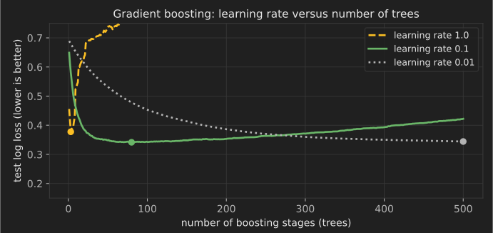
How it works: at stage , compute the negative gradient of the loss for every training example (for squared error, simply the residuals ), fit a small tree to it, and update (Friedman, 2001). The learning rate shrinks each step; smaller rates need more trees but usually generalize better. Any differentiable loss works, which is why boosting handles classification, regression, ranking and quantiles.
When to use it: the strongest general-purpose choice for tabular data. It needs more tuning than a random forest (learning rate, number of trees, depth) and early stopping to avoid overfitting.
from sklearn.datasets import load_breast_cancer
from sklearn.ensemble import GradientBoostingClassifier
from sklearn.model_selection import cross_val_score

X, y = load_breast_cancer(return_X_y=True)
model = GradientBoostingClassifier(n_estimators=200, learning_rate=0.1, max_depth=3, random_state=0)
print("mean CV accuracy:", round(cross_val_score(model, X, y, cv=5).mean(), 3))
mean CV accuracy: 0.963
Real-world application: web search ranking. Gradient-boosted trees trained with the LambdaMART ranking objective were used in production search ranking at Microsoft Bing, and an ensemble of LambdaMART models won the 2010 Yahoo! Learning to Rank Challenge (Burges, 2010).
30. Histogram-based gradient boosting (LightGBM-style)
What it is: a much faster implementation of gradient boosting that bins each feature into at most 255 buckets before training.
How it works: with binned features, finding the best split means scanning a histogram instead of sorting values, which makes training on millions of rows practical. LightGBM popularized this approach together with leaf-wise tree growth and sampling tricks (Ke et al., 2017); scikit-learn's HistGradientBoostingClassifier is inspired by it and also handles missing values and categorical features natively.
When to use it: any tabular dataset above roughly 10,000 rows; it is the boosting estimator scikit-learn recommends for larger data.
from sklearn.datasets import make_classification
from sklearn.ensemble import HistGradientBoostingClassifier
from sklearn.model_selection import train_test_split

X, y = make_classification(n_samples=100_000, n_features=30, n_informative=10, random_state=0)
X_train, X_test, y_train, y_test = train_test_split(X, y, random_state=0)
model = HistGradientBoostingClassifier(early_stopping=True, random_state=0).fit(X_train, y_train)
print("test accuracy:", round(model.score(X_test, y_test), 3), "| boosting iterations used:", model.n_iter_)
test accuracy: 0.967 | boosting iterations used: 100
Real-world application: LightGBM-style boosting is a common choice for fraud scoring, credit risk, demand forecasting and churn prediction. In the M5 retail forecasting competition, the organizers report that LightGBM was used by most of the top-ranked teams (Makridakis, Spiliotis and Assimakopoulos, 2022).
31. XGBoost
What it is: a popular gradient boosting library that adds explicit regularization and a second-order (Newton) step to each tree.
How it works: each tree is chosen to minimize a second-order Taylor approximation of the loss plus a penalty on the number of leaves and leaf weights , which gives a closed-form optimal weight per leaf (Chen and Guestrin, 2016). It also introduced sparsity-aware handling of missing values and efficient parallel and out-of-core training.
When to use it: the same problems as other boosting libraries. Once tuned, XGBoost, LightGBM and CatBoost usually perform similarly; choose by speed, categorical handling and deployment needs.
# requires: pip install xgboost (not run for this article)
from sklearn.datasets import load_breast_cancer
from sklearn.model_selection import cross_val_score
from xgboost import XGBClassifier

X, y = load_breast_cancer(return_X_y=True)
model = XGBClassifier(n_estimators=300, learning_rate=0.05, max_depth=4, reg_lambda=1.0)
print(cross_val_score(model, X, y, cv=5).mean())
Real-world application: the XGBoost paper reports that 17 of the 29 winning solutions published on Kaggle's blog in 2015 used it (Chen and Guestrin, 2016), and it is widely deployed for risk and fraud scoring.
32. CatBoost
What it is: a gradient boosting library designed around categorical features.
How it works: it encodes categories with target statistics computed over a random ordering of the rows, so each row's encoding uses only rows that come "before" it, and applies the same ordering idea to boosting itself. This avoids the target leakage that naive target encoding causes (Prokhorenkova et al., 2018). It grows symmetric (oblivious) trees, which are fast at prediction time.
When to use it: tabular data with many high-cardinality categorical columns (user IDs, product codes, cities), where it often needs less preprocessing and tuning.
# requires: pip install catboost (not run for this article)
import pandas as pd
from catboost import CatBoostClassifier

df = pd.DataFrame({"city": ["Paris", "Lyon", "Paris", "Nice"] * 50, "spend": range(200)})
y = (df["spend"] % 3 == 0).astype(int)
model = CatBoostClassifier(iterations=200, verbose=0).fit(df, y, cat_features=["city"])
print(model.predict_proba(df.head(2)))
Real-world application: CatBoost was developed and open-sourced by Yandex, which uses it in its own search, recommendation and forecasting services (CatBoost).
33. Stacking
What it is: trains a "meta-model" to combine the predictions of several different models.
How it works: produce out-of-fold predictions from each base model with cross-validation, so the meta-model never learns from predictions on rows the base models were trained on, then fit a simple model (often logistic or ridge regression) on those predictions (Wolpert, 1992).
When to use it: when you have diverse models with different error patterns and need the last bit of accuracy. It adds training and serving complexity.
from sklearn.datasets import load_breast_cancer
from sklearn.ensemble import RandomForestClassifier, StackingClassifier
from sklearn.linear_model import LogisticRegression
from sklearn.model_selection import cross_val_score
from sklearn.neighbors import KNeighborsClassifier
from sklearn.pipeline import make_pipeline
from sklearn.preprocessing import StandardScaler

X, y = load_breast_cancer(return_X_y=True)
stack = StackingClassifier(
    estimators=[("forest", RandomForestClassifier(random_state=0)),
                ("knn", make_pipeline(StandardScaler(), KNeighborsClassifier()))],
    final_estimator=LogisticRegression(max_iter=1000))
print("mean CV accuracy:", round(cross_val_score(stack, X, y, cv=5).mean(), 3))
mean CV accuracy: 0.97
Real-world application: the team that won the Netflix Prize blended the predictions of hundreds of models. Netflix later wrote that it did not put the full blend into production because the additional accuracy did not justify the engineering effort (Netflix Technology Blog, 2012).
34. Voting and averaging ensembles
What it is: combines models by a majority vote or by averaging their predicted probabilities.
How it works: hard voting takes the most common predicted class; soft voting averages probabilities, which usually works better when the models are calibrated. Averaging regression predictions works the same way. Unlike stacking, the weights are fixed rather than learned.
When to use it: a cheap, low-risk way to gain a little accuracy and stability from models you already have.
from sklearn.datasets import load_wine
from sklearn.ensemble import RandomForestClassifier, VotingClassifier
from sklearn.linear_model import LogisticRegression
from sklearn.model_selection import cross_val_score
from sklearn.naive_bayes import GaussianNB
from sklearn.pipeline import make_pipeline
from sklearn.preprocessing import StandardScaler

X, y = load_wine(return_X_y=True)
vote = VotingClassifier([("lr", make_pipeline(StandardScaler(), LogisticRegression(max_iter=1000))),
                         ("rf", RandomForestClassifier(random_state=0)), ("nb", GaussianNB())], voting="soft")
print("mean CV accuracy:", round(cross_val_score(vote, X, y, cv=5).mean(), 3))
mean CV accuracy: 0.978
Real-world application: weather forecasting combines runs of several models (multi-model ensembles), and the ensemble average is usually more accurate than any single run; machine learning ensembles apply the same principle.
35. Isolation forest
What it is: an anomaly detector that isolates unusual points with random splits.
How it works: build random trees by repeatedly picking a random feature and a random split value. Anomalies are few and different, so they get isolated after fewer splits; the anomaly score is based on the average path length needed to isolate a point (Liu, Ting and Zhou, 2008).
When to use it: unsupervised anomaly detection on tabular data with many features. It is fast and needs no distance metric, but it struggles with points that are only unusual in a specific context.
import numpy as np
from sklearn.ensemble import IsolationForest

rng = np.random.default_rng(0)
normal = rng.normal(0, 1, size=(500, 4))
odd = rng.normal(5, 1, size=(5, 4))
X = np.vstack([normal, odd])
labels = IsolationForest(contamination=0.01, random_state=0).fit_predict(X)  # -1 = anomaly
print("flagged rows:", np.where(labels == -1)[0])
flagged rows: [273 500 501 502 503 504]
The five planted anomalies (rows 500–504) are all caught. Row 273 is a normal point that happens to sit in the tail: setting contamination fixes how many rows get flagged, so on real data choose it from the review capacity you have.
Real-world application: flagging unusual transactions, server metrics or sensor readings for review, where labeled fraud or failure examples are rare or missing.
Clustering
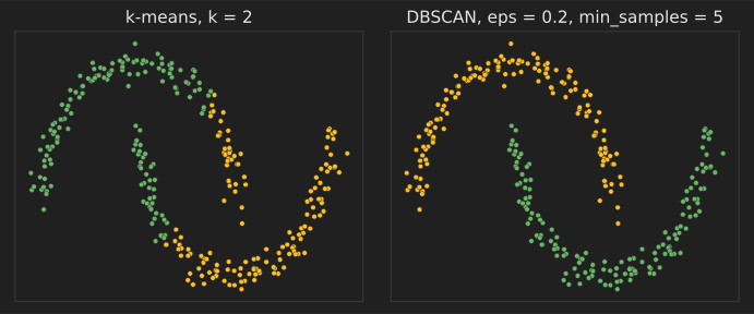
Clustering finds groups in unlabeled data. There is no single correct answer: algorithms define "group" differently (compact blobs, dense regions, connected structures), so choose the one whose definition matches your problem and check that the clusters mean something.
36. k-means
What it is: divides data into groups so that each point is close to the center of its group.
How it works: Lloyd's algorithm alternates two steps until nothing changes: assign each point to the nearest center, then move each center to the mean of its points. This minimizes the within-cluster sum of squares. The k-means++ initialization spreads the starting centers out and gives better, more consistent results (Arthur and Vassilvitskii, 2007).
When to use it: fast clustering of round, similar-sized groups in numeric data. You must choose (try silhouette scores or the elbow method), scale the features, and expect poor results on elongated or nested shapes.
from sklearn.cluster import KMeans
from sklearn.datasets import make_blobs
from sklearn.metrics import silhouette_score

X, _ = make_blobs(n_samples=600, centers=4, random_state=0)
for k in (2, 3, 4, 5, 6):
    labels = KMeans(n_clusters=k, n_init=10, random_state=0).fit_predict(X)
    print(f"k={k}: silhouette {silhouette_score(X, labels):.3f}")
k=2: silhouette 0.463
k=3: silhouette 0.467
k=4: silhouette 0.500
k=5: silhouette 0.436
k=6: silhouette 0.402
Real-world application: color quantization (reducing an image to a palette of colors), customer segmentation, and vector quantization to compress embeddings for large-scale similarity search.
37. Mini-batch k-means
What it is: k-means that updates centers from small random batches, so it scales to millions of points.
How it works: each step samples a mini-batch, assigns its points to the nearest centers and moves those centers toward the batch points with a decreasing step size (Sculley, 2010). The result is slightly worse than full k-means but much faster.
When to use it: large or streaming datasets where full k-means is too slow.
import time
from sklearn.cluster import KMeans, MiniBatchKMeans
from sklearn.datasets import make_blobs

X, _ = make_blobs(n_samples=200_000, centers=8, n_features=10, random_state=0)
for Model in (KMeans, MiniBatchKMeans):
    start = time.perf_counter()
    model = Model(n_clusters=8, n_init=3, random_state=0).fit(X)
    print(f"{Model.__name__}: inertia {model.inertia_:,.0f}, {time.perf_counter() - start:.1f} s")
KMeans: inertia 1,997,522, 0.6 s
MiniBatchKMeans: inertia 1,997,665, 0.5 s
The two inertias (within-cluster sums of squares) are almost identical. On this machine both finished in under a second; mini-batch k-means pulls ahead as datasets grow into the millions of rows or no longer fit in memory, because each step touches only a small batch.
Real-world application: Sculley's paper introduced the method for clustering web-scale data at Google, where full k-means passes over billions of examples are impractical.
38. Agglomerative hierarchical clustering
What it is: builds a tree of clusters by repeatedly merging the two closest groups.
How it works: start with every point as its own cluster. At each step, merge the pair with the smallest linkage distance: Ward linkage (smallest increase in variance), complete (farthest points), average, or single (closest points). Cutting the resulting dendrogram at a chosen height gives any number of clusters.
When to use it: small to medium datasets where the hierarchy itself is informative or the number of clusters is unknown. Standard implementations need memory.
from sklearn.cluster import AgglomerativeClustering
from sklearn.datasets import load_iris
from sklearn.metrics import adjusted_rand_score

X, y = load_iris(return_X_y=True)
for linkage in ("ward", "complete", "average", "single"):
    labels = AgglomerativeClustering(n_clusters=3, linkage=linkage).fit_predict(X)
    print(f"{linkage:8s} agreement with species (ARI): {adjusted_rand_score(y, labels):.3f}")
ward     agreement with species (ARI): 0.731
complete agreement with species (ARI): 0.642
average  agreement with species (ARI): 0.759
single   agreement with species (ARI): 0.564
Real-world application: gene-expression heat maps in biology, where hierarchical clustering of genes and samples is a standard way to show which groups behave alike (Eisen et al., 1998).
39. DBSCAN
What it is: a density-based method that finds clusters of any shape and labels sparse points as noise.
How it works: a point is a core point if at least min_samples points lie within radius . Core points within of each other join the same cluster, border points attach to a nearby core point, and everything else is noise (Ester et al., 1996).
When to use it: spatial data and irregular shapes where you do not know the number of clusters. It struggles when clusters have very different densities, and must be chosen carefully (a k-distance plot helps).
import numpy as np
from sklearn.cluster import DBSCAN
from sklearn.datasets import make_moons

X, _ = make_moons(n_samples=300, noise=0.06, random_state=0)
labels = DBSCAN(eps=0.2, min_samples=5).fit_predict(X)
print("clusters:", len(set(labels) - {-1}), "| noise points:", int(np.sum(labels == -1)))
clusters: 2 | noise points: 0
Real-world application: grouping GPS points into places (stops and frequently visited locations) and detecting clusters of events on a map, such as disease cases.
40. HDBSCAN
What it is: a hierarchical version of DBSCAN that handles clusters of different densities without choosing .
How it works: it builds the cluster hierarchy for all density levels at once (from a minimum spanning tree of "mutual reachability" distances) and keeps the clusters that persist over the widest range of densities (Campello, Moulavi and Sander, 2013). The main parameter is the minimum cluster size.
When to use it: exploratory clustering when density varies, such as clustering text or image embeddings; it is often a better default than DBSCAN.
import numpy as np
from sklearn.cluster import HDBSCAN

rng = np.random.default_rng(0)
dense = rng.normal([0, 0], 0.2, size=(200, 2))
sparse = rng.normal([4, 4], 1.0, size=(200, 2))
labels = HDBSCAN(min_cluster_size=20).fit_predict(np.vstack([dense, sparse]))
print("clusters found:", len(set(labels) - {-1}), "| noise:", int(np.sum(labels == -1)))
clusters found: 2 | noise: 0
Real-world application: topic discovery in document collections; the BERTopic library clusters sentence embeddings with HDBSCAN after reducing them with UMAP (Grootendorst, 2022).
41. OPTICS
What it is: a density-based method that orders points so clusters at every density level can be read off one plot.
How it works: OPTICS computes a reachability distance for each point in a special processing order (Ankerst et al., 1999). Valleys in the reachability plot are clusters, and deeper valleys are denser ones. Clusters can be extracted at any afterward without rerunning.
When to use it: like HDBSCAN, when densities vary and you want to inspect the structure before deciding.
import numpy as np
from sklearn.cluster import OPTICS
from sklearn.datasets import make_blobs

X, _ = make_blobs(n_samples=400, centers=[[0, 0], [5, 5], [0, 6]], cluster_std=[0.4, 1.2, 0.6], random_state=0)
labels = OPTICS(min_samples=15).fit_predict(X)
print("clusters:", len(set(labels) - {-1}), "| noise:", int(np.sum(labels == -1)))
clusters: 3 | noise: 65
Real-world application: analyzing spatial and trajectory data, such as ship or aircraft tracks, where traffic density varies widely between regions.
42. Mean shift
What it is: finds clusters by moving each point uphill to the nearest peak of the data density.
How it works: repeatedly replace each candidate point with the mean of the points within a bandwidth around it. Points that converge to the same density peak (mode) form one cluster, so the number of clusters is not fixed in advance (Comaniciu and Meer, 2002).
When to use it: low-dimensional data where clusters correspond to density peaks. It is slow on large datasets, and the bandwidth controls everything.
from sklearn.cluster import MeanShift, estimate_bandwidth
from sklearn.datasets import make_blobs

X, _ = make_blobs(n_samples=500, centers=3, cluster_std=0.7, random_state=0)
bandwidth = estimate_bandwidth(X, quantile=0.15, random_state=0)
model = MeanShift(bandwidth=bandwidth).fit(X)
print("clusters found:", len(model.cluster_centers_))
clusters found: 3
Real-world application: object tracking in video, where mean shift follows the peak of a color histogram from frame to frame, and image segmentation by color and position.
43. Gaussian mixture model (fitted with EM)
What it is: a probabilistic clustering model that treats the data as a mix of several Gaussian distributions and gives each point a probability of belonging to each one.
How it works: the expectation–maximization algorithm alternates between computing each point's responsibilities and re-estimating the weights, means and covariances from them (Dempster, Laird and Rubin, 1977). Choose the number of components with the BIC.
When to use it: clusters that are elliptical or overlap, when you need soft assignments, or as a density model for anomaly detection.
from sklearn.datasets import make_blobs
from sklearn.mixture import GaussianMixture

X, _ = make_blobs(n_samples=500, centers=3, random_state=1)
for k in (1, 2, 3, 4, 5):
    print(f"k={k}: BIC {GaussianMixture(n_components=k, random_state=0).fit(X).bic(X):.0f}")
gmm = GaussianMixture(n_components=3, random_state=0).fit(X)
print("membership probabilities of first point:", gmm.predict_proba(X[:1]).round(3))
k=1: BIC 5478
k=2: BIC 4185
k=3: BIC 3988
k=4: BIC 4017
k=5: BIC 4054
membership probabilities of first point: [[0. 0. 1.]]
The lowest BIC marks the preferred number of components.
Real-world application: classic speaker-verification systems modeled each voice as a Gaussian mixture over audio features (Reynolds, Quatieri and Dunn, 2000), and Gaussian mixtures are used for background subtraction in video.
44. Spectral clustering
What it is: clusters points by their connections in a similarity graph rather than by distance to a center.
How it works: build a similarity graph (for example, nearest neighbors), compute the leading eigenvectors of its graph Laplacian, and run k-means in that eigenvector space (Ng, Jordan and Weiss, 2001). Connected but non-convex shapes become easy to separate.
When to use it: small to medium datasets with complex shapes, and graph data. The eigen-decomposition limits scalability.
from sklearn.cluster import KMeans, SpectralClustering
from sklearn.datasets import make_circles
from sklearn.metrics import adjusted_rand_score

X, y = make_circles(n_samples=400, factor=0.4, noise=0.05, random_state=0)
km = KMeans(n_clusters=2, n_init=10, random_state=0).fit_predict(X)
sc = SpectralClustering(n_clusters=2, affinity="nearest_neighbors", random_state=0).fit_predict(X)
print("k-means ARI:", round(adjusted_rand_score(y, km), 3), "| spectral ARI:", round(adjusted_rand_score(y, sc), 3))
k-means ARI: -0.002 | spectral ARI: 1.0
Real-world application: image segmentation, where the normalized-cuts method splits an image into regions by cutting a graph of similar neighboring pixels (Shi and Malik, 2000).
45. BIRCH
What it is: a clustering method that compresses a large dataset into a tree of small summaries in a single pass.
How it works: each node of the clustering-feature tree stores only the count, linear sum and squared sum of the points it absorbs, which is enough to compute centroids and radii (Zhang, Ramakrishnan and Livny, 1996). A final clustering step runs on the leaf summaries.
When to use it: very large numeric datasets, or as a fast pre-clustering step.
from sklearn.cluster import Birch
from sklearn.datasets import make_blobs

X, _ = make_blobs(n_samples=100_000, centers=5, random_state=0)
model = Birch(threshold=0.5, n_clusters=5).fit(X)
print("leaf subclusters:", len(model.subcluster_centers_), "| final clusters:", len(set(model.labels_)))
leaf subclusters: 214 | final clusters: 5
Real-world application: pre-clustering large customer or sensor datasets before a more expensive analysis, which is how the original paper framed it for very large databases.
46. Affinity propagation
What it is: picks actual data points as cluster "exemplars" by passing messages between points.
How it works: points exchange "responsibility" (how well suited is to be 's exemplar) and "availability" (how appropriate it would be for to choose ) messages until a set of exemplars emerges (Frey and Dueck, 2007). The number of clusters follows from a "preference" value, not a fixed .
When to use it: small datasets where you want representative examples. Memory and time grow with . The preference value controls how many exemplars appear: with scikit-learn's default (the median similarity) this data splits into many small clusters, so the snippet sets it lower.
from sklearn.cluster import AffinityPropagation
from sklearn.datasets import make_blobs

X, _ = make_blobs(n_samples=300, centers=4, cluster_std=0.6, random_state=0)
model = AffinityPropagation(preference=-50, random_state=0).fit(X)
print("clusters:", len(model.cluster_centers_indices_), "| exemplar rows:", model.cluster_centers_indices_)
clusters: 4 | exemplar rows: [158 192 206 259]
Real-world application: the original paper used it to pick representative sentences for summarizing a manuscript and to identify cities that would make efficient airline hubs.
Dimensionality reduction and representation learning
These methods compress many features into a few, to visualize data, remove noise, speed up other models or discover hidden factors. Linear methods (PCA, SVD, NMF) are fast and interpretable; non-linear ones (t-SNE, UMAP, autoencoders) capture curved structure.
47. Principal component analysis (PCA)
What it is: rotates the data onto new axes ordered by how much variance they capture, then keeps the first few.
How it works: center the data and compute its singular value decomposition . The rows of are the principal directions, and the share of variance explained by component is . Projecting onto the top directions gives the best rank- approximation in squared error.
When to use it: to visualize high-dimensional data, decorrelate features, remove noise, or speed up models. Scale features first if their units differ. Components are linear and can be hard to name.
from sklearn.datasets import load_digits
from sklearn.decomposition import PCA

X, _ = load_digits(return_X_y=True)
pca = PCA().fit(X)
cumulative = pca.explained_variance_ratio_.cumsum()
print("components for 90% of variance:", int((cumulative < 0.90).sum()) + 1, "of", X.shape[1])
components for 90% of variance: 21 of 64
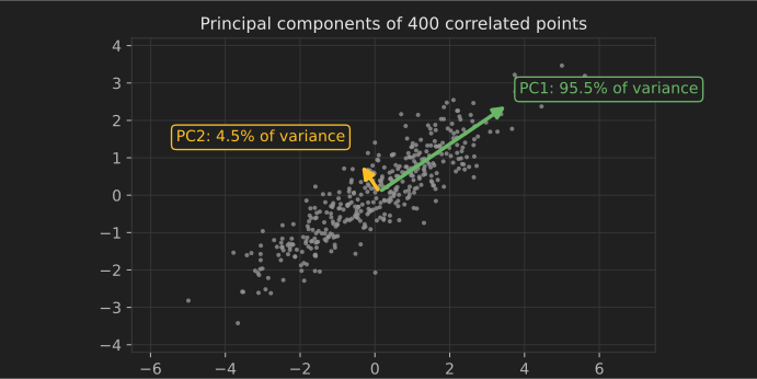
Real-world application: population genetics, where PCA of genotype data reveals ancestry; in a well-known study, the first two components of European genomes closely mirrored a map of Europe (Novembre et al., 2008).
48. Kernel PCA
What it is: PCA with the kernel trick, so it can unfold curved structure.
How it works: performs PCA on the centered kernel matrix instead of on the covariance matrix (Schölkopf, Smola and Müller, 1998). With an RBF kernel, concentric circles can become separable along a single component.
When to use it: non-linear structure in small to medium datasets; the kernel matrix is .
from sklearn.datasets import make_circles
from sklearn.decomposition import PCA, KernelPCA
from sklearn.linear_model import LogisticRegression
from sklearn.model_selection import cross_val_score
from sklearn.pipeline import make_pipeline

X, y = make_circles(n_samples=400, factor=0.3, noise=0.05, random_state=0)
for reducer in (PCA(n_components=1), KernelPCA(n_components=1, kernel="rbf", gamma=5)):
    acc = cross_val_score(make_pipeline(reducer, LogisticRegression()), X, y, cv=5).mean()
    print(f"{type(reducer).__name__}: accuracy with 1 component {acc:.3f}")
PCA: accuracy with 1 component 0.460
KernelPCA: accuracy with 1 component 1.000
Real-world application: non-linear process monitoring in chemical plants, where kernel PCA models normal operation and faults show up as large deviations in the kernel component space.
49. Truncated SVD (latent semantic analysis)
What it is: a low-rank SVD that works directly on large sparse matrices, such as document–word counts.
How it works: computes only the top singular vectors of (without centering, so sparsity is preserved) using randomized or iterative solvers. Applied to a TF-IDF matrix it is called latent semantic analysis: documents and words that co-occur end up close together in the reduced space (Deerwester et al., 1990).
When to use it: reducing sparse text or interaction matrices before clustering or classification.
from sklearn.decomposition import TruncatedSVD
from sklearn.feature_extraction.text import TfidfVectorizer

docs = ["the cat sat on the mat", "dogs and cats are pets", "stock markets fell today",
        "investors sold shares", "my pet dog chased the cat", "shares and stocks rose"]
X = TfidfVectorizer().fit_transform(docs)
Z = TruncatedSVD(n_components=2, random_state=0).fit_transform(X)
print(Z.round(2))
[[ 0.82  0.  ]
 [-0.    0.48]
 [ 0.    0.  ]
 [-0.    0.64]
 [ 0.82  0.  ]
 [-0.    0.8 ]]
Real-world application: information retrieval systems used LSA to match queries to documents that share meaning but not exact words, which was its original purpose.
50. Independent component analysis (ICA)
What it is: separates a mixed signal into statistically independent sources.
How it works: assumes the observations are linear mixtures of independent, non-Gaussian sources, and finds an unmixing matrix that makes the recovered components as non-Gaussian as possible. FastICA does this with a fixed-point iteration (Hyvärinen and Oja, 2000).
When to use it: blind source separation of signals: audio, EEG, financial factors. It cannot recover the order or scale of the sources.
import numpy as np
from sklearn.decomposition import FastICA

t = np.linspace(0, 8, 2000)
sources = np.c_[np.sin(2 * t), np.sign(np.sin(3 * t))]          # a sine and a square wave
mixed = sources @ np.array([[1.0, 0.5], [0.4, 1.0]]).T          # two "microphones"
recovered = FastICA(n_components=2, random_state=0).fit_transform(mixed)
corr = np.abs(np.corrcoef(sources.T, recovered.T)[:2, 2:])
print("best |correlation| of each source with a component:", corr.max(axis=1).round(3))
best |correlation| of each source with a component: [0.998 1. ]
Real-world application: removing eye-blink and muscle artifacts from EEG recordings, a standard step in neuroscience toolkits (Jung et al., 2000).
51. Non-negative matrix factorization (NMF)
What it is: factors a non-negative matrix into two smaller non-negative matrices, which tends to produce additive, parts-based components.
How it works: finds with by minimizing a reconstruction loss with multiplicative or coordinate-descent updates (Lee and Seung, 1999). Because nothing can be subtracted, each component is a "part": a topic, a facial feature, a spectral signature.
When to use it: counts, intensities and spectra, when interpretable components matter. Results depend on initialization.
from sklearn.decomposition import NMF
from sklearn.feature_extraction.text import TfidfVectorizer

docs = ["goal match team score", "team players won the match", "election vote party",
        "the party won the vote", "striker scored a goal", "voters and candidates"]
vec = TfidfVectorizer(stop_words="english")
nmf = NMF(n_components=2, random_state=0).fit(vec.fit_transform(docs))
words = vec.get_feature_names_out()
for i, comp in enumerate(nmf.components_):
    print(f"topic {i}:", [str(words[j]) for j in comp.argsort()[-3:][::-1]])
topic 0: ['vote', 'party', 'election']
topic 1: ['team', 'match', 'goal']
Real-world application: mutational-signature analysis in cancer genomics, where NMF decomposes tumor mutation counts into signatures linked to causes such as tobacco smoke or ultraviolet light (Alexandrov et al., 2013).
52. Factor analysis
What it is: models observed variables as driven by a few hidden factors plus variable-specific noise.
How it works: assumes with and independent noise whose variance differs per variable. Unlike PCA, it separates shared variance from each variable's own noise.
When to use it: survey and psychometric data, where you want the latent traits behind many questions.
import numpy as np
from sklearn.decomposition import FactorAnalysis

rng = np.random.default_rng(0)
traits = rng.normal(size=(500, 2))                              # two hidden traits
loadings = np.array([[1, 0], [0.9, 0], [0.8, 0.1], [0, 1], [0.1, 0.9], [0, 0.8]])
answers = traits @ loadings.T + rng.normal(0, 0.3, size=(500, 6))
fa = FactorAnalysis(n_components=2, rotation="varimax", random_state=0).fit(answers)
print(np.abs(fa.components_).round(2))
[[0.96 0.87 0.81 0.01 0.1  0.01]
 [0.03 0.01 0.08 0.97 0.89 0.78]]
Each recovered factor loads on one block of three questions, matching how the data was generated.
Real-world application: the "Big Five" personality traits emerged from factor analyses of personality questionnaires, and factor models are standard in finance for explaining asset returns.
53. Latent Dirichlet allocation (topic model)
What it is: a probabilistic model that describes each document as a mixture of topics and each topic as a distribution over words.
How it works: assumes each document draws topic proportions from a Dirichlet distribution and each word from one of those topics (Blei, Ng and Jordan, 2003). Variational inference or Gibbs sampling estimates the topics from word counts.
When to use it: exploring large text collections when you want interpretable topics. Results need human review, and embedding-based topic methods often give more coherent topics on short texts.
from sklearn.decomposition import LatentDirichletAllocation
from sklearn.feature_extraction.text import CountVectorizer

docs = ["bank loan interest rate", "interest rates and loans", "river bank fishing boat",
        "boat trip on the river", "mortgage loan bank", "fishing on the lake by boat",
        "loan interest mortgage rate", "boat fishing lake river"]
vec = CountVectorizer(stop_words="english")
lda = LatentDirichletAllocation(n_components=2, max_iter=50, random_state=0).fit(vec.fit_transform(docs))
words = vec.get_feature_names_out()
for i, comp in enumerate(lda.components_):
    print(f"topic {i}:", [str(words[j]) for j in comp.argsort()[-4:][::-1]])
topic 0: ['loan', 'bank', 'rate', 'mortgage']
topic 1: ['boat', 'fishing', 'river', 'lake']
Real-world application: digital humanities and social science research, such as tracking topics across decades of newspaper archives, scientific abstracts or parliamentary speeches.
54. t-SNE
What it is: a visualization method that places similar high-dimensional points close together in two or three dimensions.
How it works: converts distances into neighbor probabilities in the original space and in the map, then moves map points to minimize the KL divergence between the two, using a heavy-tailed Student-t distribution in the map to avoid crowding (van der Maaten and Hinton, 2008).
When to use it: visual exploration only. Cluster sizes and distances between clusters in a t-SNE plot are not meaningful, results change with perplexity and the random seed, and it cannot embed new points.
from sklearn.datasets import load_digits
from sklearn.manifold import TSNE
from sklearn.neighbors import KNeighborsClassifier

X, y = load_digits(return_X_y=True)
Z = TSNE(n_components=2, perplexity=30, random_state=0).fit_transform(X)
knn = KNeighborsClassifier(5).fit(Z, y)
print("map shape:", Z.shape, "| share of points whose map neighbors match their digit:", round(knn.score(Z, y), 3))
map shape: (1797, 2) | share of points whose map neighbors match their digit: 0.99
Real-world application: visualizing single-cell RNA sequencing data, where each point is a cell and t-SNE or UMAP maps reveal cell types.
55. UMAP
What it is: a faster non-linear embedding method that often preserves more global structure than t-SNE.
How it works: builds a weighted nearest-neighbor graph in the original space, then optimizes a low-dimensional layout whose graph matches it, using a cross-entropy objective (McInnes, Healy and Melville, 2018). It can transform new points and can embed into more than three dimensions as preprocessing for clustering.
When to use it: visualization, and as a step before density-based clustering of embeddings. As with t-SNE, do not over-interpret distances.
# requires: pip install umap-learn (not run for this article)
import umap
from sklearn.datasets import load_digits

X, y = load_digits(return_X_y=True)
Z = umap.UMAP(n_neighbors=15, min_dist=0.1, random_state=0).fit_transform(X)
print(Z.shape)
Real-world application: single-cell biology, where UMAP plots quickly became a standard figure (Becht et al., 2019), and exploring embeddings of documents or images.
56. Isomap
What it is: a non-linear embedding that preserves distances measured along the data's surface.
How it works: connect each point to its nearest neighbors, compute shortest-path (geodesic) distances through this graph, then apply classical multidimensional scaling to those distances (Tenenbaum, de Silva and Langford, 2000).
When to use it: data that lies on a smooth surface (a manifold), such as images of an object under continuously varying pose. It is sensitive to noise and to "short circuits" between nearby folds.
from scipy.stats import spearmanr
from sklearn.datasets import make_swiss_roll
from sklearn.manifold import Isomap

X, t = make_swiss_roll(n_samples=1000, random_state=0)   # t = position along the roll
Z = Isomap(n_neighbors=10, n_components=2).fit_transform(X)
print("rank correlation of first Isomap axis with roll position:", round(abs(spearmanr(Z[:, 0], t)[0]), 3))
rank correlation of first Isomap axis with roll position: 1.0
Real-world application: the original paper recovered pose and lighting directions from collections of face images, and the method is used to analyze motion-capture and other continuously varying signals.
57. Locally linear embedding (LLE)
What it is: a non-linear embedding that preserves how each point is reconstructed from its neighbors.
How it works: express each point as a weighted combination of its nearest neighbors, then find low-dimensional coordinates that keep the same weights (Roweis and Saul, 2000). It only needs local geometry, so it can unroll curved surfaces.
When to use it: smooth manifolds with dense sampling. It is sensitive to the number of neighbors and to noise.
from scipy.stats import spearmanr
from sklearn.datasets import make_s_curve
from sklearn.manifold import LocallyLinearEmbedding

X, t = make_s_curve(n_samples=1000, random_state=0)
Z = LocallyLinearEmbedding(n_neighbors=12, n_components=2, random_state=0).fit_transform(X)
print("rank correlation with position along the curve:", round(max(abs(spearmanr(Z[:, i], t)[0]) for i in range(2)), 3))
rank correlation with position along the curve: 1.0
Real-world application: research on face images and speech features, where high-dimensional signals vary along a few underlying parameters such as expression or pitch.
58. Random projection
What it is: reduces dimensions by multiplying the data by a random matrix.
How it works: the Johnson–Lindenstrauss lemma guarantees that projecting points into random dimensions keeps all pairwise distances within a factor of with high probability (Dasgupta and Gupta, 2003). No fitting is needed.
When to use it: very high-dimensional data (text, hashed features) where PCA is too slow and approximate distances are enough.
import numpy as np
from sklearn.metrics import pairwise_distances
from sklearn.random_projection import GaussianRandomProjection

rng = np.random.default_rng(0)
X = rng.normal(size=(300, 10_000))
Z = GaussianRandomProjection(n_components=1000, random_state=0).fit_transform(X)
upper = np.triu_indices(300, 1)
ratio = pairwise_distances(Z)[upper] / pairwise_distances(X)[upper]
print(f"distance ratio after projection: min {ratio.min():.3f}, max {ratio.max():.3f}")
distance ratio after projection: min 0.918, max 1.115
Real-world application: locality-sensitive hashing for near-duplicate detection of web pages and images uses random projections to put similar items in the same bucket.
Anomaly detection
Anomaly detectors learn what "normal" looks like and flag points that do not fit. Isolation forest (entry 35) belongs here too. Labeled anomalies are usually rare, so evaluation relies on a small labeled sample or expert review.
59. Local outlier factor (LOF)
What it is: flags points that sit in much sparser regions than their neighbors.
How it works: compares each point's local density, based on distances to its nearest neighbors, with the densities of those neighbors (Breunig et al., 2000). A ratio well above 1 means the point is less dense than its surroundings, so outliers are judged relative to local context.
When to use it: data where normal density varies by region, so a single global threshold would fail.
import numpy as np
from sklearn.neighbors import LocalOutlierFactor

rng = np.random.default_rng(0)
dense = rng.normal(0, 0.3, size=(200, 2))
sparse = rng.normal(5, 2.0, size=(200, 2))
outlier = np.array([[1.5, 1.5]])                    # near the dense cluster but outside it
X = np.vstack([dense, sparse, outlier])
labels = LocalOutlierFactor(n_neighbors=20, contamination=0.01).fit_predict(X)
print("last point flagged:", bool(labels[-1] == -1))
last point flagged: True
Real-world application: network intrusion detection and fraud review, where activity that is normal for one user or segment is suspicious for another.
60. One-class SVM
What it is: learns a boundary around normal data using only normal examples.
How it works: maps data with a kernel and finds the hyperplane that separates the data from the origin with maximum margin; nu bounds the fraction of training points treated as outliers (Schölkopf et al., 2001).
When to use it: novelty detection when you have clean normal data and moderate dataset sizes. It is sensitive to gamma and to feature scaling.
import numpy as np
from sklearn.svm import OneClassSVM

rng = np.random.default_rng(0)
normal = rng.normal(0, 1, size=(300, 2))
model = OneClassSVM(kernel="rbf", nu=0.05, gamma=0.5).fit(normal)
print(model.predict([[0, 0], [0.5, -0.5], [4, 4]]))  # 1 = normal, -1 = novelty
[ 1 1 -1]
Real-world application: monitoring machines with vibration or acoustic sensors, where failures are rare and the model is trained on healthy operation only.
61. Elliptic envelope (robust covariance)
What it is: fits a robust Gaussian ellipse to the data and flags points far outside it.
How it works: estimates the mean and covariance with the minimum covariance determinant method, which ignores a fraction of extreme points (Rousseeuw and Van Driessen, 1999), then scores points by Mahalanobis distance .
When to use it: roughly Gaussian, low-dimensional data, such as a few correlated process measurements.
import numpy as np
from sklearn.covariance import EllipticEnvelope

rng = np.random.default_rng(0)
X = rng.multivariate_normal([0, 0], [[1, 0.9], [0.9, 1]], size=300)
model = EllipticEnvelope(contamination=0.02, random_state=0).fit(X)
print(model.predict([[1, 1], [1, -1]]))   # (1, -1) breaks the correlation
[ 1 -1]
Both test points are the same distance from the center, but breaks the strong correlation between the two variables, so its Mahalanobis distance is large and it is flagged.
Real-world application: multivariate statistical process control in manufacturing, where a combination of readings can be abnormal even when each reading is within its own limits.
Association rules and recommender systems
These algorithms find items that go together and predict what a user will like next.
62. Apriori (association rules)
What it is: finds sets of items that frequently appear together in transactions and turns them into rules such as "bread and butter → milk".
How it works: uses the fact that every subset of a frequent itemset must also be frequent, so candidates of size are built only from frequent sets of size (Agrawal and Srikant, 1994). Rules are ranked by support (how often the items occur together), confidence and lift .
When to use it: market-basket analysis on transaction data. FP-growth is faster on large datasets (the mlxtend library implements both). The snippet below counts item pairs directly, which is the first level of Apriori.
from collections import Counter
from itertools import combinations

baskets = [{"bread", "milk"}, {"bread", "butter", "milk"}, {"beer", "chips"},
           {"bread", "butter"}, {"bread", "butter", "milk"}, {"beer", "chips", "bread"}]
n = len(baskets)
pairs = Counter(pair for b in baskets for pair in combinations(sorted(b), 2))
singles = Counter(item for b in baskets for item in b)
for (a, b), count in pairs.most_common(3):
    print(f"{a} -> {b}: support {count / n:.2f}, confidence {count / singles[a]:.2f}, "
          f"lift {(count / singles[a]) / (singles[b] / n):.2f}")
bread -> milk: support 0.50, confidence 0.60, lift 1.20
bread -> butter: support 0.50, confidence 0.60, lift 1.20
butter -> milk: support 0.33, confidence 0.67, lift 1.33
A lift above 1 means the items appear together more often than if they were independent.
Real-world application: product placement, bundles and "frequently bought together" suggestions in retail, and finding co-occurring diagnoses or prescriptions in health records.
63. Item-based collaborative filtering
What it is: recommends items similar to the ones a user already liked, where similarity comes from other users' behavior.
How it works: represent each item by the vector of ratings or interactions it received, compute item–item cosine similarities, and score an unseen item for a user by a similarity-weighted average of their ratings (Sarwar et al., 2001). Item similarities are stable and can be precomputed.
When to use it: catalogs with plenty of interaction data. It cannot recommend new items with no interactions (the cold-start problem).
import numpy as np

# rows = users, columns = items A-D (0 = not rated)
R = np.array([[5, 4, 0, 1], [4, 5, 1, 0], [1, 0, 5, 4], [0, 1, 4, 5], [5, 0, 0, 1]], dtype=float)
norms = np.linalg.norm(R, axis=0)
S = (R.T @ R) / np.outer(norms, norms)          # item-item cosine similarity
user = R[4]                                      # rated A=5 and D=1
scores = S @ user / (np.abs(S) @ (user > 0))
scores[user > 0] = -np.inf
print("recommend item:", "ABCD"[int(np.argmax(scores))], "| scores:", np.round(scores, 2))
recommend item: B | scores: [-inf 4.12 1.61 -inf]
Real-world application: Amazon's "customers who bought this item also bought" recommendations were built on item-to-item collaborative filtering (Linden, Smith and York, 2003).
64. Matrix factorization (alternating least squares)
What it is: learns a short vector for every user and every item so that their dot product predicts the rating or preference.
How it works: approximate the sparse rating matrix by , minimizing squared error on observed entries plus L2 penalties. Alternating least squares fixes and solves a ridge regression for each user, then fixes and solves one for each item (Koren, Bell and Volinsky, 2009). Implicit-feedback variants weight clicks and views by a confidence value (Hu, Koren and Volinsky, 2008).
When to use it: large recommendation problems with many users and items. Like other collaborative methods, it needs side features or content to handle new users and items.
import numpy as np

rng = np.random.default_rng(0)
true_u, true_v = rng.normal(size=(50, 3)), rng.normal(size=(40, 3))
R = true_u @ true_v.T
mask = rng.random(R.shape) < 0.3                       # only 30% of ratings observed
k, lam = 3, 0.1
U, V = rng.normal(size=(50, k)), rng.normal(size=(40, k))
for _ in range(20):
    for i in range(50):
        Vi = V[mask[i]]
        U[i] = np.linalg.solve(Vi.T @ Vi + lam * np.eye(k), Vi.T @ R[i, mask[i]])
    for j in range(40):
        Uj = U[mask[:, j]]
        V[j] = np.linalg.solve(Uj.T @ Uj + lam * np.eye(k), Uj.T @ R[mask[:, j], j])
rmse = np.sqrt(np.mean((U @ V.T - R)[~mask] ** 2))
print(f"RMSE on the 70% of ratings never seen: {rmse:.3f} (ratings have std {R.std():.2f})")
RMSE on the 70% of ratings never seen: 0.115 (ratings have std 1.74)
Real-world application: matrix factorization was central to the leading Netflix Prize solutions and became a standard recommendation technique; Apache Spark's MLlib ships an ALS implementation for large-scale implicit feedback (Spark documentation).
Time series and sequential models
Time-ordered data breaks the assumption that rows are independent, so it needs models that use the order and evaluation that respects it: always validate on a period after the training period, never on randomly shuffled rows.
65. Autoregressive models and ARIMA
What it is: predicts the next value of a series from its own recent values (autoregression), its recent forecast errors (moving average) and, after differencing, its trend (the "I" in ARIMA).
How it works: an AR() model is . ARIMA() differences the series times to remove trend and adds lagged error terms, following the Box–Jenkins method of identifying, fitting and checking the model (Box and Jenkins, 1970). The snippet fits an AR(2) model by least squares with NumPy; in practice you would use statsmodels.tsa.arima.model.ARIMA.
When to use it: short-term forecasts of a single, reasonably stable series. It handles one series at a time and assumes the dynamics do not change.
import numpy as np

rng = np.random.default_rng(0)
y = np.zeros(500)
for t in range(2, 500):
    y[t] = 0.6 * y[t - 1] - 0.3 * y[t - 2] + rng.normal()
X = np.c_[y[1:-1], y[:-2]]                   # lags 1 and 2
phi, *_ = np.linalg.lstsq(X, y[2:], rcond=None)
print("estimated coefficients:", phi.round(3), "(true 0.6 and -0.3)")
print("one-step forecast:", round(float(phi @ [y[-1], y[-2]]), 3))
estimated coefficients: [ 0.598 -0.327] (true 0.6 and -0.3)
one-step forecast: 0.583
Real-world application: official statistics. The U.S. Census Bureau's X-13ARIMA-SEATS program, which uses ARIMA models to extend series before seasonal adjustment, is used by statistical agencies to publish seasonally adjusted figures (U.S. Census Bureau).
66. Exponential smoothing (Holt–Winters)
What it is: forecasts with a weighted average of past observations, where the weights decay exponentially into the past.
How it works: simple exponential smoothing updates the level . Holt's method adds a trend term, and Holt–Winters adds a seasonal term, each with its own smoothing parameter (Hyndman and Athanasopoulos, Forecasting: Principles and Practice).
When to use it: many series that need cheap, robust forecasts with trend and seasonality. In the M3 forecasting competition, simple methods such as exponential smoothing were hard to beat (Makridakis and Hibon, 2000).
import numpy as np

def holt(y, alpha=0.5, beta=0.2, horizon=3):
    level, trend = y[0], y[1] - y[0]
    for value in y[1:]:
        prev_level = level
        level = alpha * value + (1 - alpha) * (level + trend)
        trend = beta * (level - prev_level) + (1 - beta) * trend
    return [level + h * trend for h in range(1, horizon + 1)]

rng = np.random.default_rng(0)
sales = 100 + 2 * np.arange(40) + rng.normal(0, 3, 40)   # upward trend plus noise
print("next three forecasts:", np.round(holt(sales), 1), "| true trend values:", 100 + 2 * np.arange(40, 43))
next three forecasts: [183.4 186. 188.5] | true trend values: [180 182 184]
Real-world application: inventory and replenishment systems that forecast demand for thousands of products, where exponential smoothing remains a common default because it is fast, stable and easy to monitor.
67. Kalman filter
What it is: estimates the hidden state of a moving system (such as position and velocity) from noisy measurements, updating the estimate as each new measurement arrives.
How it works: alternates a predict step, which moves the state forward with a linear model and increases its uncertainty, and an update step, which blends the prediction with the new measurement in proportion to their uncertainties via the Kalman gain (Kalman, 1960). For linear systems with Gaussian noise it is the optimal estimator.
When to use it: tracking and sensor fusion. Extended and unscented variants handle non-linear systems; particle filters handle non-Gaussian ones.
import numpy as np

rng = np.random.default_rng(0)
dt, steps = 1.0, 100
F = np.array([[1, dt], [0, 1]]); H = np.array([[1.0, 0.0]])
Q, R = 0.01 * np.eye(2), np.array([[4.0]])
true = np.zeros((steps, 2)); true[0] = [0, 1]
for t in range(1, steps):
    true[t] = F @ true[t - 1] + rng.multivariate_normal([0, 0], Q)
measured = true[:, 0] + rng.normal(0, 2, steps)
x, P, estimates = np.array([0.0, 0.0]), 10 * np.eye(2), []
for z in measured:
    x, P = F @ x, F @ P @ F.T + Q                       # predict
    K = P @ H.T @ np.linalg.inv(H @ P @ H.T + R)        # Kalman gain
    x, P = x + K @ (z - H @ x), (np.eye(2) - K @ H) @ P  # update
    estimates.append(x[0])
rmse = lambda a: np.sqrt(np.mean((np.array(a) - true[:, 0]) ** 2))
print(f"position error: raw sensor {rmse(measured):.2f}, Kalman filter {rmse(estimates):.2f}")
position error: raw sensor 2.23, Kalman filter 1.00
Real-world application: navigation. Kalman filtering was used in the Apollo navigation computer and is now standard in aircraft, spacecraft, GPS receivers and phones that fuse satellite positions with motion sensors (Grewal and Andrews, 2010).
68. Hidden Markov model (with the Viterbi algorithm)
What it is: a model of a sequence driven by hidden states that switch according to fixed probabilities, where each state produces observations with its own distribution.
How it works: an HMM has initial, transition and emission probabilities. The forward algorithm computes the probability of a sequence, Baum–Welch (a form of EM) learns the parameters, and the Viterbi algorithm finds the most likely hidden-state path by dynamic programming (Rabiner, 1989).
When to use it: sequences with a small number of regimes, such as speech sounds, gene regions or market states, especially when you want an interpretable model. Deep sequence models have replaced HMMs where data is plentiful.
import numpy as np

# A casino switches between a fair die and a loaded die that rolls 6 half the time.
start = np.log([0.5, 0.5])
trans = np.log([[0.95, 0.05], [0.10, 0.90]])
emit = np.log([[1 / 6] * 6, [0.1] * 5 + [0.5]])
rolls = [int(c) - 1 for c in "3152463125466666366566661524312"]
score = start + emit[:, rolls[0]]
back = []
for r in rolls[1:]:
    cand = score[:, None] + trans                       # previous state x next state
    back.append(cand.argmax(axis=0))
    score = cand.max(axis=0) + emit[:, r]
path = [int(score.argmax())]
for b in reversed(back):
    path.append(int(b[path[-1]]))
print("rolls: ", "".join(str(r + 1) for r in rolls))
print("states:", "".join("FL"[s] for s in reversed(path)), "(F = fair, L = loaded)")
rolls:  3152463125466666366566661524312
states: FFFFFFFFFFFLLLLLLLLLLLLLFFFFFFF (F = fair, L = loaded)
Real-world application: speech recognition systems were built on HMMs for decades, and gene-finding programs such as GENSCAN used them to label DNA as exons, introns and other regions (Burge and Karlin, 1997).
69. Dynamic time warping (DTW)
What it is: measures the similarity of two sequences that may be shifted or stretched in time.
How it works: finds the alignment between the two sequences that minimizes the total distance, allowing one point to match several, by dynamic programming over a cost matrix: (Sakoe and Chiba, 1978).
When to use it: comparing or classifying time series whose speed varies, such as gestures, spoken words or sensor traces. A 1-nearest-neighbor classifier with DTW is a strong baseline for time-series classification. It costs per pair, so constrain the warping window on long series.
import numpy as np

def dtw(a, b):
    D = np.full((len(a) + 1, len(b) + 1), np.inf)
    D[0, 0] = 0
    for i in range(1, len(a) + 1):
        for j in range(1, len(b) + 1):
            D[i, j] = abs(a[i - 1] - b[j - 1]) + min(D[i - 1, j], D[i, j - 1], D[i - 1, j - 1])
    return D[-1, -1]

t = np.linspace(0, 2 * np.pi, 60)
a, shifted, different = np.sin(t), np.sin(t - 0.6), np.cos(2 * t)
print("Euclidean: shifted", round(np.abs(a - shifted).sum(), 1), "| different", round(np.abs(a - different).sum(), 1))
print("DTW:       shifted", round(dtw(a, shifted), 1), "| different", round(dtw(a, different), 1))
Euclidean: shifted 22.8 | different 49.8
DTW:       shifted 5.0 | different 21.7
DTW sees the shifted sine wave as nearly identical, while plain point-by-point distance treats it as quite different.
Real-world application: the original DTW paper was about recognizing spoken words; the method is still used in signature verification, gesture recognition and matching sensor traces from wearables.
Semi-supervised learning
When labels are expensive but unlabeled data is plentiful, semi-supervised methods use the structure of the unlabeled data to spread the few labels you have.
70. Label propagation and label spreading
What it is: spreads known labels to unlabeled points through a similarity graph, on the idea that nearby points probably share a label.
How it works: build a graph over all points, labeled and unlabeled, then iteratively let each node take on a weighted average of its neighbors' label distributions while the labeled nodes stay anchored (Zhu and Ghahramani, 2002; Zhou et al., 2004). Label spreading adds regularization so noisy labels can change.
When to use it: when a few labels exist and the classes form clusters in feature space.
import numpy as np
from sklearn.datasets import load_digits
from sklearn.semi_supervised import LabelSpreading

X, y = load_digits(return_X_y=True)
rng = np.random.default_rng(0)
y_partial = np.full_like(y, -1)                       # -1 marks unlabeled rows
labeled = rng.choice(len(y), size=50, replace=False)  # keep only 50 of 1,797 labels
y_partial[labeled] = y[labeled]
model = LabelSpreading(kernel="knn", n_neighbors=7).fit(X, y_partial)
unlabeled = y_partial == -1
print("accuracy on the unlabeled rows:", round((model.transduction_[unlabeled] == y[unlabeled]).mean(), 3))
accuracy on the unlabeled rows: 0.903
Real-world application: speeding up the labeling of large image, text or medical-record collections: experts label a small seed set, propagation proposes labels for the rest, and humans review the uncertain cases.
71. Self-training (pseudo-labeling)
What it is: trains a model on the labeled data, uses it to label the unlabeled data it is most confident about, and retrains on both.
How it works: repeat: fit, predict probabilities on unlabeled rows, add rows above a confidence threshold with their predicted labels, and refit (Yarowsky, 1995). Errors can reinforce themselves, so use a high threshold and check on a labeled validation set.
When to use it: any classifier with reasonably calibrated probabilities and lots of unlabeled data from the same distribution. The snippet shows both outcomes: self-training helps the logistic regression but hurts the random forest, whose confident mistakes get added as labels.
import numpy as np
from sklearn.datasets import load_digits
from sklearn.ensemble import RandomForestClassifier
from sklearn.linear_model import LogisticRegression
from sklearn.model_selection import train_test_split
from sklearn.pipeline import make_pipeline
from sklearn.preprocessing import StandardScaler
from sklearn.semi_supervised import SelfTrainingClassifier

X, y = load_digits(return_X_y=True)
X_train, X_test, y_train, y_test = train_test_split(X, y, random_state=0)
rng = np.random.default_rng(0)
y_partial = y_train.copy()
y_partial[rng.random(len(y_partial)) > 0.05] = -1     # keep about 5% of the labels
labeled = y_partial != -1
for name, base in [("logistic regression", make_pipeline(StandardScaler(), LogisticRegression(max_iter=2000))),
                   ("random forest", RandomForestClassifier(n_estimators=300, random_state=0))]:
    only_labeled = base.fit(X_train[labeled], y_partial[labeled]).score(X_test, y_test)
    self_trained = SelfTrainingClassifier(base, threshold=0.9).fit(X_train, y_partial).score(X_test, y_test)
    print(f"{name}: labeled rows only {only_labeled:.3f} | with self-training {self_trained:.3f}")
logistic regression: labeled rows only 0.822 | with self-training 0.889
random forest: labeled rows only 0.807 | with self-training 0.782
Real-world application: the Noisy Student method used a teacher model to pseudo-label 300 million unlabeled images, improving ImageNet accuracy over training on labeled images alone (Xie et al., 2020).
Neural networks and deep learning
Neural networks stack simple layers of weighted sums and non-linear functions, trained end to end with gradient descent and backpropagation. They learn their own features from raw inputs, which is why they dominate images, audio and language. The PyTorch snippets below are deliberately tiny so they run on a CPU in seconds; real models use the same building blocks at much larger scale.
72. Perceptron
What it is: the original artificial neuron: a linear classifier trained by nudging the weights whenever it makes a mistake.
How it works: predict ; for each misclassified example, update (Rosenblatt, 1958). If the classes are linearly separable, it is guaranteed to converge.
When to use it: mainly for teaching and as a fast online linear classifier. It cannot solve non-linear problems such as XOR, which is the limitation that multi-layer networks overcame.
import numpy as np
from sklearn.linear_model import Perceptron

X = np.array([[0, 0], [0, 1], [1, 0], [1, 1]])
for name, y in [("AND", [0, 0, 0, 1]), ("XOR", [0, 1, 1, 0])]:
    accuracy = Perceptron(max_iter=100, random_state=0).fit(X, y).score(X, y)
    print(f"{name}: training accuracy {accuracy:.2f}")
AND: training accuracy 1.00
XOR: training accuracy 0.50
Real-world application: today the perceptron's main role is as the conceptual building block of every neural network layer; Rosenblatt's Mark I Perceptron was built in the late 1950s to recognize simple images from a camera.
73. Multilayer perceptron and backpropagation
What it is: a network of fully connected layers with non-linear activations, trained by backpropagation.
How it works: each layer computes with an activation such as ReLU. Backpropagation applies the chain rule from the loss back through each layer to get every weight's gradient in one backward pass, and an optimizer updates the weights (Rumelhart, Hinton and Williams, 1986).
When to use it: a general-purpose non-linear model, and the final layers of most deep networks. On tabular data, tuned boosted trees usually beat plain MLPs.
import torch
from sklearn.datasets import load_digits
from sklearn.model_selection import train_test_split

torch.manual_seed(0)
X, y = load_digits(return_X_y=True)
X_train, X_test, y_train, y_test = train_test_split(X / 16.0, y, random_state=0)
X_train, X_test = torch.tensor(X_train, dtype=torch.float32), torch.tensor(X_test, dtype=torch.float32)
y_train, y_test = torch.tensor(y_train), torch.tensor(y_test)
model = torch.nn.Sequential(torch.nn.Linear(64, 64), torch.nn.ReLU(), torch.nn.Linear(64, 10))
opt = torch.optim.Adam(model.parameters(), lr=0.01)
for epoch in range(100):
    opt.zero_grad()
    loss = torch.nn.functional.cross_entropy(model(X_train), y_train)
    loss.backward()                                   # backpropagation
    opt.step()
accuracy = (model(X_test).argmax(1) == y_test).float().mean().item()
print(f"final training loss {loss.item():.3f} | test accuracy {accuracy:.3f}")
final training loss 0.027 | test accuracy 0.969
Real-world application: ALVINN, an early self-driving project at Carnegie Mellon, used a small fully connected network trained with backpropagation to steer a vehicle from camera images (Pomerleau, 1988).
74. Adam optimizer
What it is: the most widely used optimizer for training neural networks; it adapts a separate step size for every weight.
How it works: keeps exponential moving averages of the gradient and of its square , corrects them for their zero initialization, and updates (Kingma and Ba, 2014). Weights with consistently small gradients get relatively larger steps. AdamW decouples weight decay from the update (Loshchilov and Hutter, 2017).
When to use it: the default for most deep learning. Plain SGD with momentum sometimes generalizes better for image classification when well tuned. For the theory, see optimization techniques.
import torch

def run(optimizer_cls, **kwargs):
    w = torch.tensor([-1.5, 2.0], requires_grad=True)
    opt = optimizer_cls([w], **kwargs)
    for _ in range(2000):
        opt.zero_grad()
        loss = (1 - w[0]) ** 2 + 100 * (w[1] - w[0] ** 2) ** 2   # Rosenbrock valley, minimum at (1, 1)
        loss.backward()
        opt.step()
    return f"loss {loss.item():.4f} at {w.detach().numpy().round(3)}"

print("SGD: ", run(torch.optim.SGD, lr=1e-4))     # larger SGD steps diverge on this function
print("Adam:", run(torch.optim.Adam, lr=0.05))
SGD:  loss 5.3382 at [-1.309  1.721]
Adam: loss 0.0000 at [1. 1.]
Real-world application: large language models and most modern vision models are trained with Adam or AdamW; for example, the GPT-3 paper reports training with Adam (Brown et al., 2020).
75. Convolutional neural network (CNN)
What it is: a network that scans images with small learned filters, so it detects the same pattern anywhere in the image.
How it works: a convolution layer slides each filter across the input and computes dot products, producing feature maps; pooling layers downsample them. Sharing filter weights across positions gives translation equivariance and far fewer parameters than a fully connected layer (LeCun et al., 1998). Stacked layers detect edges, then textures, then parts, then objects.
When to use it: images, and other grid-like signals such as spectrograms. Vision transformers compete at large scale, but CNNs remain efficient and strong, especially with limited data.
import torch
from sklearn.datasets import load_digits
from sklearn.model_selection import train_test_split

torch.manual_seed(0)
X, y = load_digits(return_X_y=True)
X = torch.tensor(X / 16.0, dtype=torch.float32).reshape(-1, 1, 8, 8)
X_train, X_test, y_train, y_test = train_test_split(X, torch.tensor(y), random_state=0)
model = torch.nn.Sequential(
    torch.nn.Conv2d(1, 16, 3, padding=1), torch.nn.ReLU(), torch.nn.MaxPool2d(2),   # 16 x 4 x 4
    torch.nn.Conv2d(16, 32, 3, padding=1), torch.nn.ReLU(), torch.nn.MaxPool2d(2),  # 32 x 2 x 2
    torch.nn.Flatten(), torch.nn.Linear(128, 10))
opt = torch.optim.Adam(model.parameters(), lr=0.01)
for epoch in range(60):
    opt.zero_grad()
    torch.nn.functional.cross_entropy(model(X_train), y_train).backward()
    opt.step()
print("test accuracy:", round((model(X_test).argmax(1) == y_test).float().mean().item(), 3))
test accuracy: 0.984
Real-world application: LeCun's convolutional networks were deployed to read handwritten amounts on bank checks in the 1990s, and CNNs now power medical image analysis, quality inspection and the camera features in phones.
76. Residual network (ResNet)
What it is: a very deep network made trainable by adding "skip connections" that let each block learn a correction to its input.
How it works: each block outputs instead of (He et al., 2015). The identity path lets gradients flow straight back through dozens or hundreds of layers, which avoids the vanishing gradients that stop plain deep networks from training. The snippet compares the gradient reaching the first layer of a 50-layer network with and without skip connections.
When to use it: any deep network; residual connections are now part of nearly every large architecture, including transformers.
import torch

torch.manual_seed(0)
x = torch.randn(64, 32)
layers = [torch.nn.Linear(32, 32) for _ in range(50)]
for residual in (False, True):
    h = x
    for layer in layers:
        out = torch.tanh(layer(h))
        h = h + out if residual else out
    for layer in layers:
        layer.weight.grad = None
    h.pow(2).mean().backward()
    print(f"residual={residual}: gradient norm at first layer {layers[0].weight.grad.norm().item():.2e}")
residual=False: gradient norm at first layer 4.81e-14
residual=True: gradient norm at first layer 1.33e+01
Real-world application: ResNets won the 2015 ImageNet classification challenge and became the standard backbone for image classification, object detection and medical-imaging models.
77. U-Net
What it is: an encoder–decoder network for image segmentation: it labels every pixel.
How it works: the encoder downsamples to capture context, the decoder upsamples back to full resolution, and skip connections copy high-resolution features from each encoder level to the matching decoder level so fine boundaries are kept (Ronneberger, Fischer and Brox, 2015). The snippet trains a tiny two-level U-Net to find bright squares in noisy images.
When to use it: pixel-level tasks: medical segmentation, satellite land-cover mapping, defect localization. The same architecture is used as the denoiser in many diffusion models.
import torch
import torch.nn as nn

torch.manual_seed(0)

def batch(n=32, size=32):
    images, masks = torch.randn(n, 1, size, size) * 0.5, torch.zeros(n, 1, size, size)
    for i in range(n):
        r, c, s = torch.randint(0, 20, (2,)).tolist() + [torch.randint(6, 12, (1,)).item()]
        images[i, 0, r:r + s, c:c + s] += 1.5
        masks[i, 0, r:r + s, c:c + s] = 1
    return images, masks

class TinyUNet(nn.Module):
    def __init__(self):
        super().__init__()
        self.enc1 = nn.Sequential(nn.Conv2d(1, 8, 3, padding=1), nn.ReLU())
        self.enc2 = nn.Sequential(nn.MaxPool2d(2), nn.Conv2d(8, 16, 3, padding=1), nn.ReLU())
        self.up = nn.ConvTranspose2d(16, 8, 2, stride=2)
        self.dec = nn.Sequential(nn.Conv2d(16, 8, 3, padding=1), nn.ReLU(), nn.Conv2d(8, 1, 1))
    def forward(self, x):
        e1 = self.enc1(x)
        e2 = self.enc2(e1)
        return self.dec(torch.cat([self.up(e2), e1], dim=1))   # skip connection

model, loss_fn = TinyUNet(), nn.BCEWithLogitsLoss()
opt = torch.optim.Adam(model.parameters(), lr=0.01)
for step in range(200):
    images, masks = batch()
    opt.zero_grad(); loss_fn(model(images), masks).backward(); opt.step()
images, masks = batch(64)
pred = model(images) > 0
iou = ((pred & (masks > 0)).sum() / (pred | (masks > 0)).sum()).item()
print(f"intersection over union on new images: {iou:.3f}")
intersection over union on new images: 0.992
Real-world application: U-Net variants are standard in biomedical segmentation; the self-configuring nnU-Net framework set state-of-the-art results across many medical segmentation challenges (Isensee et al., 2021).
78. Recurrent neural network (RNN)
What it is: a network that reads a sequence one step at a time and carries a hidden state forward as memory.
How it works: at each step, , and outputs are computed from (Elman, 1990). Training unrolls the network through time and backpropagates through every step, which makes gradients vanish or explode over long sequences.
When to use it: short sequences, or as a teaching step toward LSTMs and GRUs. For most sequence tasks, gated RNNs or transformers work better.
import torch

torch.manual_seed(0)
t = torch.linspace(0, 40, 801)
wave = torch.sin(t)
X = torch.stack([wave[i:i + 20] for i in range(760)]).unsqueeze(-1)   # windows of 20 steps
y = wave[20:780].unsqueeze(-1)                                         # the next value
rnn, head = torch.nn.RNN(1, 16, batch_first=True), torch.nn.Linear(16, 1)
opt = torch.optim.Adam(list(rnn.parameters()) + list(head.parameters()), lr=0.01)
for epoch in range(150):
    opt.zero_grad()
    out, _ = rnn(X)
    loss = torch.nn.functional.mse_loss(head(out[:, -1]), y)
    loss.backward()
    opt.step()
print(f"mean squared error predicting the next point: {loss.item():.5f}")
mean squared error predicting the next point: 0.00009
Real-world application: recurrent networks were the basis of neural language models and early neural machine translation before LSTMs and then transformers took over.
79. Long short-term memory (LSTM)
What it is: a recurrent network with gates that decide what to remember, forget and output, so it can keep information over long sequences.
How it works: a separate cell state is updated additively, , where the forget gate , input gate and output gate are sigmoid functions of the input and previous state (Hochreiter and Schmidhuber, 1997). The additive path keeps gradients from vanishing, especially when the forget-gate bias starts at a positive value so the cell remembers by default, a standard initialization trick (Jozefowicz, Zaremba and Sutskever, 2015). The snippet asks a network to recall the sign of the first number in a sequence of 50 noisy numbers.
When to use it: sequence tasks with long-range dependencies when data or compute is too limited for a transformer, and streaming tasks that must process one step at a time.
import torch

def task(n=64, length=50):
    x = torch.randn(n, length, 1) * 0.2
    sign = torch.randint(0, 2, (n,))
    x[:, 0, 0] = sign * 2.0 - 1.0          # the only informative step is the first one
    return x, sign

for Cell in (torch.nn.RNN, torch.nn.LSTM):
    torch.manual_seed(0)
    cell, head = Cell(1, 16, batch_first=True), torch.nn.Linear(16, 2)
    if Cell is torch.nn.LSTM:
        with torch.no_grad():
            cell.bias_ih_l0[16:32].fill_(3.0)   # forget-gate bias: remember by default
    opt = torch.optim.Adam(list(cell.parameters()) + list(head.parameters()), lr=0.01)
    for step in range(400):
        x, y = task()
        opt.zero_grad()
        torch.nn.functional.cross_entropy(head(cell(x)[0][:, -1]), y).backward()
        opt.step()
    x, y = task(2000)
    print(f"{Cell.__name__}: accuracy {(head(cell(x)[0][:, -1]).argmax(1) == y).float().mean().item():.3f}")
RNN: accuracy 0.496
LSTM: accuracy 1.000
The plain RNN stays at chance (50%) because the gradient from the last step back to the first one vanishes. In our runs, an LSTM with PyTorch's default initialization also failed to learn this task within the same budget, which is why the forget-gate bias matters.
Real-world application: Google's neural machine translation system, launched in 2016, was built on deep LSTM encoder–decoder networks (Wu et al., 2016), and LSTMs were widely used in speech recognition and keyboard prediction.
80. Gated recurrent unit (GRU)
What it is: a simpler gated RNN with two gates instead of three and no separate cell state.
How it works: an update gate blends the old state with a candidate state, , and a reset gate controls how much of the past feeds the candidate (Cho et al., 2014). It has about three quarters of an LSTM's parameters and often performs similarly.
When to use it: the same problems as LSTMs, when you want a smaller, faster model; try both.
import torch

lstm, gru = torch.nn.LSTM(32, 64), torch.nn.GRU(32, 64)
count = lambda m: sum(p.numel() for p in m.parameters())
print(f"parameters with 32 inputs and 64 hidden units: LSTM {count(lstm):,}, GRU {count(gru):,}")
parameters with 32 inputs and 64 hidden units: LSTM 25,088, GRU 18,816
Real-world application: compact GRU and LSTM models are used for on-device sequence tasks such as wake-word detection and sensor-based activity recognition, where model size and latency are tight.
81. Self-attention and the transformer
What it is: the architecture behind modern language models. Instead of reading a sequence step by step, every position looks directly at every other position.
How it works: each token is projected into a query , key and value . Attention computes : each output is a weighted average of the values, with weights from query–key similarity (Vaswani et al., 2017). Multiple heads run in parallel, and blocks of attention plus feed-forward layers are stacked with residual connections and normalization. Because there is no recurrence, training parallelizes across the sequence. See linear algebra for machine learning for the matrix view.
When to use it: language, code and, increasingly, images, audio, proteins and time series, especially with large datasets or pretrained models. Attention costs grow with the square of sequence length.
import torch
import torch.nn.functional as F

torch.manual_seed(0)
x = torch.randn(1, 5, 16)                               # 1 sequence, 5 tokens, 16 dimensions
Wq, Wk, Wv = (torch.randn(16, 16) * 0.25 for _ in range(3))
Q, K, V = x @ Wq, x @ Wk, x @ Wv
weights = torch.softmax(Q @ K.transpose(-2, -1) / 16 ** 0.5, dim=-1)
manual = weights @ V
print("attention weights for token 0:", weights[0, 0].detach().numpy().round(3))
print("matches PyTorch's built-in:", torch.allclose(manual, F.scaled_dot_product_attention(Q, K, V), atol=1e-6))
attention weights for token 0: [0.125 0.461 0.206 0.125 0.082]
matches PyTorch's built-in: True
Real-world application: transformers underlie large language models, machine translation services and code assistants, as well as AlphaFold 2's protein structure predictions, whose network is built around attention (Jumper et al., 2021).
82. BERT (masked language model pretraining)
What it is: a transformer encoder pretrained to fill in hidden words, which gives representations of text that can be fine-tuned for many tasks.
How it works: randomly select 15% of tokens; replace 80% of them with a [MASK] token, 10% with a random token and leave 10% unchanged, then train the model to predict the original tokens from context on both sides (Devlin et al., 2018). A small task-specific head is then fine-tuned on labeled data. The snippet shows the masking step; training a real BERT needs a large corpus (the Hugging Face transformers library provides pretrained models).
When to use it: text classification, named-entity recognition, search relevance and other language-understanding tasks, especially with modest labeled data. For generating text, decoder models (next entry) are used instead.
import random

random.seed(1)
tokens = "the model reads the whole sentence before predicting the hidden word".split()
vocab = sorted(set(tokens))
masked, targets = [], {}
for i, tok in enumerate(tokens):
    if random.random() < 0.15:
        targets[i] = tok
        r = random.random()
        masked.append("[MASK]" if r < 0.8 else random.choice(vocab) if r < 0.9 else tok)
    else:
        masked.append(tok)
print(" ".join(masked))
print("positions the model must predict:", targets)
hidden model reads the whole sentence [MASK] predicting the hidden [MASK]
positions the model must predict: {0: 'the', 6: 'before', 10: 'word'}
Real-world application: in 2019 Google said it had started using BERT models in Search to better understand queries, initially for about one in ten English searches in the U.S. (Google, 2019).
83. GPT-style autoregressive language model
What it is: a transformer decoder trained to predict the next token, which can then generate text one token at a time.
How it works: a causal mask stops each position from attending to later positions, and the model minimizes the cross-entropy of every next token (Radford et al., 2018). Scaled up, this one objective produces models that can follow instructions after further fine-tuning (Brown et al., 2020). The snippet trains a one-layer character-level model on a repeated phrase and then generates from a prompt.
When to use it: text and code generation, chat assistants, summarization and any task that can be phrased as text in, text out. In practice you use a pretrained model rather than training one.
import torch
import torch.nn as nn

torch.manual_seed(0)
text = "machine learning learns from data. " * 30
chars = sorted(set(text)); idx = {c: i for i, c in enumerate(chars)}
data = torch.tensor([idx[c] for c in text])
block, d = 32, 64

class TinyGPT(nn.Module):
    def __init__(self):
        super().__init__()
        self.tok, self.pos = nn.Embedding(len(chars), d), nn.Embedding(block, d)
        self.block = nn.TransformerEncoderLayer(d, nhead=4, dim_feedforward=128, batch_first=True)
        self.out = nn.Linear(d, len(chars))
    def forward(self, x):
        mask = nn.Transformer.generate_square_subsequent_mask(x.shape[1])   # causal mask
        h = self.tok(x) + self.pos(torch.arange(x.shape[1]))
        return self.out(self.block(h, src_mask=mask, is_causal=True))

model = TinyGPT()
opt = torch.optim.Adam(model.parameters(), lr=3e-3)
for step in range(300):
    starts = torch.randint(0, len(data) - block - 1, (32,))
    x = torch.stack([data[s:s + block] for s in starts]); y = torch.stack([data[s + 1:s + block + 1] for s in starts])
    opt.zero_grad(); nn.functional.cross_entropy(model(x).transpose(1, 2), y).backward(); opt.step()
model.eval()
out = [idx[c] for c in "machine "]
with torch.no_grad():
    for _ in range(40):
        logits = model(torch.tensor([out[-block:]]))[0, -1]
        out.append(int(logits.argmax()))
print("".join(chars[i] for i in out))
machine learning learns from data. machine learn
Real-world application: chat assistants, code completion tools and document-drafting features in office software are built on large autoregressive transformers.
84. Word2vec (skip-gram embeddings)
What it is: learns a dense vector for each word so that words used in similar contexts get similar vectors.
How it works: the skip-gram model predicts the words around each word; with negative sampling it learns to score real (word, context) pairs above random pairs, and the learned input vectors are the embeddings (Mikolov et al., 2013). The same idea works for any sequence of items, such as products in a shopping session.
When to use it: building item or word embeddings from co-occurrence data for search, recommendations and as features for other models. Contextual embeddings from transformers have replaced it for most language tasks.
import itertools
import random
import torch

random.seed(0); torch.manual_seed(0)
pets = "cat dog pet fur paw kitten puppy".split()
money = "stock bond market price trade shares fund".split()
sentences = [random.sample(pets, 5) for _ in range(200)] + [random.sample(money, 5) for _ in range(200)]
words = sorted(set(pets + money)); idx = {w: i for i, w in enumerate(words)}
pairs = [(idx[s[i]], idx[s[j]]) for s in sentences
         for i in range(len(s)) for j in range(max(0, i - 2), min(len(s), i + 3)) if i != j]
center, context = torch.tensor(pairs).T
emb_in, emb_out = torch.nn.Embedding(len(words), 8), torch.nn.Embedding(len(words), 8)
opt = torch.optim.Adam(list(emb_in.parameters()) + list(emb_out.parameters()), lr=0.02)
for step in range(1000):
    negative = torch.randint(0, len(words), (len(center), 5))           # 5 random "noise" words per pair
    pos = (emb_in(center) * emb_out(context)).sum(1)
    neg = (emb_in(center)[:, None] * emb_out(negative)).sum(-1)
    loss = -(torch.nn.functional.logsigmoid(pos).mean() + torch.nn.functional.logsigmoid(-neg).mean())
    opt.zero_grad(); loss.backward(); opt.step()
v = torch.nn.functional.normalize(emb_in.weight, dim=1)
sim = lambda a, b: (v[idx[a]] @ v[idx[b]]).item()
within = [sim(a, b) for group in (pets, money) for a, b in itertools.combinations(group, 2)]
across = [sim(a, b) for a in pets for b in money]
print(f"mean cosine similarity within a topic {sum(within) / len(within):.2f} | across topics {sum(across) / len(across):.2f}")
mean cosine similarity within a topic 0.52 | across topics -0.03
Real-world application: Airbnb trained skip-gram embeddings on sequences of listings that users clicked in a session and used them for similar-listing recommendations and real-time search personalization (Grbovic and Cheng, 2018).
85. Autoencoder
What it is: a network trained to reproduce its input through a narrow bottleneck, so the bottleneck learns a compressed representation.
How it works: an encoder maps to a short code , a decoder maps back to , and training minimizes reconstruction error (Hinton and Salakhutdinov, 2006). With linear layers it recovers the same subspace as PCA; non-linear layers can capture curved structure.
When to use it: non-linear compression, denoising, and anomaly detection, where inputs the model reconstructs poorly are unusual.
import torch
from sklearn.datasets import load_digits
from sklearn.decomposition import PCA

torch.manual_seed(0)
X = torch.tensor(load_digits().data / 16.0, dtype=torch.float32)
model = torch.nn.Sequential(torch.nn.Linear(64, 32), torch.nn.ReLU(), torch.nn.Linear(32, 8),   # encoder
                            torch.nn.Linear(8, 32), torch.nn.ReLU(), torch.nn.Linear(32, 64))   # decoder
opt = torch.optim.Adam(model.parameters(), lr=0.005)
for epoch in range(800):
    opt.zero_grad()
    loss = torch.nn.functional.mse_loss(model(X), X)
    loss.backward()
    opt.step()
pca = PCA(n_components=8).fit(X.numpy())
pca_error = ((pca.inverse_transform(pca.transform(X.numpy())) - X.numpy()) ** 2).mean()
print(f"reconstruction error with an 8-number code: autoencoder {loss.item():.4f}, PCA {pca_error:.4f}")
reconstruction error with an 8-number code: autoencoder 0.0173, PCA 0.0239
This compares training error only; on held-out data the gap is usually smaller.
Real-world application: visual inspection in manufacturing, where an autoencoder trained only on images of good parts flags parts it cannot reconstruct well as possible defects.
86. Variational autoencoder (VAE)
What it is: an autoencoder whose code is a probability distribution, which makes it a generative model you can sample new data from.
How it works: the encoder outputs a mean and variance for ; a sample is drawn with the reparameterization trick ; and training maximizes the evidence lower bound, which is reconstruction quality minus the KL divergence between the code distribution and a standard normal prior (Kingma and Welling, 2013). Decoding samples from the prior generates new examples.
When to use it: generative modeling with a smooth, structured latent space, such as interpolating between examples or searching for designs. Samples tend to be blurrier than those of GANs or diffusion models.
import torch
from sklearn.datasets import load_digits

torch.manual_seed(0)
X = torch.tensor(load_digits().data / 16.0, dtype=torch.float32)
enc, dec = torch.nn.Linear(64, 2 * 4), torch.nn.Sequential(torch.nn.Linear(4, 64), torch.nn.Sigmoid())
opt = torch.optim.Adam(list(enc.parameters()) + list(dec.parameters()), lr=0.01)
for epoch in range(500):
    mu, log_var = enc(X).chunk(2, dim=1)
    z = mu + torch.exp(0.5 * log_var) * torch.randn_like(mu)              # reparameterization trick
    recon = torch.nn.functional.binary_cross_entropy(dec(z), X, reduction="sum") / len(X)
    kl = -0.5 * torch.sum(1 + log_var - mu ** 2 - log_var.exp()) / len(X)
    opt.zero_grad(); (recon + kl).backward(); opt.step()
samples = dec(torch.randn(5, 4))                                          # generate from the prior
print(f"reconstruction term {recon.item():.1f}, KL term {kl.item():.1f}, generated shape {tuple(samples.shape)}")
reconstruction term 23.7, KL term 3.2, generated shape (5, 64)
Real-world application: in drug discovery, VAEs trained on molecules give a continuous latent space in which researchers can search for molecules with desired properties (Gómez-Bombarelli et al., 2018); latent diffusion image generators also use a VAE to compress images.
87. Generative adversarial network (GAN)
What it is: two networks trained against each other: a generator that makes fake samples and a discriminator that tries to tell them from real ones.
How it works: the discriminator maximizes its classification accuracy and the generator minimizes it, a minimax game (Goodfellow et al., 2014). At equilibrium, generated samples follow the data distribution. Training can be unstable and can collapse onto a few modes.
When to use it: sharp image synthesis, super-resolution and image-to-image translation. Diffusion models have overtaken GANs for most image generation, but GANs are faster at sampling.
import torch

torch.manual_seed(0)
real = lambda n: torch.randn(n, 1) * 1.25 + 4.0           # target: normal with mean 4, std 1.25
G = torch.nn.Sequential(torch.nn.Linear(4, 32), torch.nn.LeakyReLU(0.2), torch.nn.Linear(32, 32),
                        torch.nn.LeakyReLU(0.2), torch.nn.Linear(32, 1))
D = torch.nn.Sequential(torch.nn.Linear(1, 32), torch.nn.LeakyReLU(0.2), torch.nn.Linear(32, 1))
opt_g = torch.optim.Adam(G.parameters(), lr=1e-3, betas=(0.5, 0.999))
opt_d = torch.optim.Adam(D.parameters(), lr=1e-3, betas=(0.5, 0.999))
bce = torch.nn.functional.binary_cross_entropy_with_logits
for step in range(3000):
    fake = G(torch.randn(128, 4))
    d_loss = bce(D(real(128)), torch.ones(128, 1)) + bce(D(fake.detach()), torch.zeros(128, 1))
    opt_d.zero_grad(); d_loss.backward(); opt_d.step()
    g_loss = bce(D(fake), torch.ones(128, 1))              # generator wants D to say "real"
    opt_g.zero_grad(); g_loss.backward(); opt_g.step()
samples = G(torch.randn(10_000, 4))
print(f"generated mean {samples.mean().item():.2f}, std {samples.std().item():.2f} (target 4.00, 1.25)")
generated mean 3.93, std 1.49 (target 4.00, 1.25)
The mean is learned quickly, but the spread keeps oscillating around the target as the two networks chase each other; in our runs it ranged from well below to above 1.25 depending on the learning rates and number of steps. That instability is typical of GAN training.
Real-world application: StyleGAN produced the first widely seen photorealistic synthetic faces (Karras, Laine and Aila, 2018); GANs are also used for image super-resolution and to synthesize training data.
88. Diffusion model
What it is: a generative model that learns to reverse a gradual noising process, turning pure noise into a sample step by step.
How it works: the forward process adds Gaussian noise over steps until the data is noise. A network is trained to predict the noise in a noisy sample, , and sampling runs the learned denoising from step down to 0 (Ho, Jain and Abbeel, 2020). The snippet learns a one-dimensional distribution with two peaks.
When to use it: high-quality image, audio, video and molecule generation. Sampling needs many network evaluations, though distillation and faster samplers reduce this.
import torch

torch.manual_seed(0)
T = 100
betas = torch.linspace(1e-4, 0.05, T)
alpha_bar = torch.cumprod(1 - betas, dim=0)
data = lambda n: torch.where(torch.rand(n, 1) < 0.5, -2.0, 2.0) + 0.3 * torch.randn(n, 1)   # two peaks
net = torch.nn.Sequential(torch.nn.Linear(2, 64), torch.nn.ReLU(), torch.nn.Linear(64, 64), torch.nn.ReLU(),
                          torch.nn.Linear(64, 1))
opt = torch.optim.Adam(net.parameters(), lr=2e-3)
for step in range(3000):
    x0, t = data(256), torch.randint(0, T, (256, 1))
    noise = torch.randn_like(x0)
    xt = alpha_bar[t].sqrt() * x0 + (1 - alpha_bar[t]).sqrt() * noise           # forward (noising) process
    loss = ((net(torch.cat([xt, t / T], 1)) - noise) ** 2).mean()                  # predict the noise
    opt.zero_grad(); loss.backward(); opt.step()
x = torch.randn(5000, 1)
with torch.no_grad():
    for t in reversed(range(T)):                                                   # reverse (denoising) process
        eps = net(torch.cat([x, torch.full_like(x, t / T)], 1))
        x = (x - betas[t] / (1 - alpha_bar[t]).sqrt() * eps) / (1 - betas[t]).sqrt()
        if t > 0:
            x += betas[t].sqrt() * torch.randn_like(x)
print(f"share of samples near -2: {(x < 0).float().mean().item():.2f} | mean |x|: {x.abs().mean().item():.2f} (data: 0.50, 2.00)")
share of samples near -2: 0.46 | mean |x|: 2.02 (data: 0.50, 2.00)
Real-world application: image generators such as Stable Diffusion are latent diffusion models, which run the diffusion process in a compressed latent space (Rombach et al., 2022).
89. Graph neural network (graph convolutional network)
What it is: a network that learns from data organized as a graph, such as social networks, molecules or road maps.
How it works: each layer updates every node from its neighbors. In a graph convolutional network, , where is the adjacency matrix with self-loops, normalized by node degree (Kipf and Welling, 2016). After layers, each node's representation reflects its -hop neighborhood. The snippet labels the members of Zachary's karate club network from just two labeled nodes.
When to use it: node classification, link prediction and whole-graph prediction (for example, molecular properties). Very deep GNNs tend to "over-smooth" node representations.
import networkx as nx
import torch

torch.manual_seed(0)
G = nx.karate_club_graph()                               # 34 members, two factions after a split
labels = torch.tensor([0 if G.nodes[n]["club"] == "Mr. Hi" else 1 for n in G.nodes])
A = torch.tensor(nx.to_numpy_array(G), dtype=torch.float32) + torch.eye(34)
d = A.sum(1).rsqrt()
A_hat = d[:, None] * A * d[None, :]                      # symmetric normalization
X = torch.eye(34)                                         # no node features: identity
W1, W2 = torch.nn.Linear(34, 16), torch.nn.Linear(16, 2)
opt = torch.optim.Adam(list(W1.parameters()) + list(W2.parameters()), lr=0.01, weight_decay=5e-4)
train = torch.tensor([0, 33])                              # only the two leaders are labeled
for epoch in range(200):
    logits = A_hat @ W2(torch.relu(A_hat @ W1(X)))
    loss = torch.nn.functional.cross_entropy(logits[train], labels[train])
    opt.zero_grad(); loss.backward(); opt.step()
accuracy = (logits.argmax(1) == labels).float().mean().item()
print(f"members assigned to the right faction: {accuracy:.2f}")
members assigned to the right faction: 0.97
Real-world application: Pinterest's PinSage graph network generated recommendations over a graph of billions of pins and boards (Ying et al., 2018), and Google Maps uses graph neural networks to predict travel times (Derrow-Pinion et al., 2021).
Reinforcement learning and sequential decision-making
Reinforcement learning (RL) learns by trial and error: an agent takes actions, receives rewards and improves its policy to maximize total reward. The simplest case, the multi-armed bandit, has one decision repeated many times; full RL adds states that change in response to actions. The standard reference is Sutton and Barto's Reinforcement Learning: An Introduction, free online.
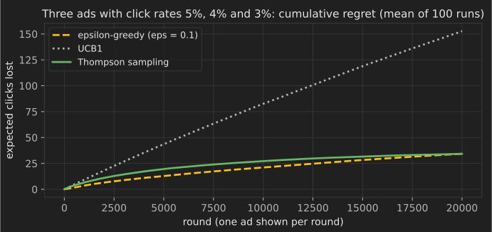
90. Epsilon-greedy bandit
What it is: the simplest way to balance trying new options (exploration) with using the best one so far (exploitation).
How it works: with probability pick a random option; otherwise pick the option with the highest average reward so far. A decaying explores less as estimates improve.
When to use it: simple online experiments where you want to shift traffic toward better options during the test. Constant keeps wasting a fixed share of traffic forever.
import numpy as np

rng = np.random.default_rng(0)
p = np.array([0.05, 0.04, 0.03])                 # true click rates of three ads (unknown to the agent)
n, wins = np.zeros(3), np.zeros(3)
for t in range(10_000):
    arm = rng.integers(3) if rng.random() < 0.1 else int(np.argmax(wins / np.maximum(n, 1)))
    n[arm] += 1
    wins[arm] += rng.random() < p[arm]
print("times each ad was shown:", n.astype(int), "| estimated rates:", (wins / n).round(3))
times each ad was shown: [9101 385 514] | estimated rates: [0.045 0.042 0.037]
Real-world application: a common baseline in online experimentation and recommendation systems that adapt as user feedback arrives.
91. Upper confidence bound (UCB1)
What it is: a bandit algorithm that is optimistic in the face of uncertainty: it picks the option whose plausible best-case reward is highest.
How it works: choose the arm maximizing , the average reward plus a bonus that shrinks as the arm is tried more (Auer, Cesa-Bianchi and Fischer, 2002). Rarely tried arms get explored; clearly bad arms are dropped. Its regret grows only logarithmically with time.
When to use it: bandit problems where you want deterministic behavior and theoretical guarantees. Contextual versions such as LinUCB use features of the user and the item. UCB1's bonus does not depend on how noisy rewards are, so with click rates of a few percent it explores far too much (see the snippet and the chart); variants such as KL-UCB use tighter bounds for that case (Garivier and Cappé, 2011).
import numpy as np

rng = np.random.default_rng(0)
p = np.array([0.05, 0.04, 0.03])
n, wins = np.ones(3), (rng.random(3) < p).astype(float)   # try each arm once
for t in range(3, 10_000):
    arm = int(np.argmax(wins / n + np.sqrt(2 * np.log(t) / n)))
    n[arm] += 1
    wins[arm] += rng.random() < p[arm]
print("times each ad was shown:", n.astype(int))
times each ad was shown: [4058 3450 2492]
Real-world application: Yahoo! used a contextual UCB algorithm (LinUCB) to personalize news articles on its front page and reported a 12.5% click lift over a context-free bandit in its evaluation (Li et al., 2010).
92. Thompson sampling
What it is: a Bayesian bandit algorithm that chooses each option with the probability that it is the best.
How it works: keep a posterior distribution for each option's reward rate (for click data, a Beta distribution updated with successes and failures), draw one sample from each posterior, and play the option with the highest sample (Thompson, 1933). Uncertain options sometimes produce high samples, so exploration happens automatically.
When to use it: most practical bandit problems; it is simple, handles delayed feedback well and usually performs at least as well as UCB.
import numpy as np

rng = np.random.default_rng(0)
p = np.array([0.05, 0.04, 0.03])
wins, losses = np.zeros(3), np.zeros(3)
for t in range(10_000):
    arm = int(np.argmax(rng.beta(1 + wins, 1 + losses)))   # one posterior sample per ad
    click = rng.random() < p[arm]
    wins[arm] += click
    losses[arm] += 1 - click
print("times each ad was shown:", (wins + losses).astype(int))
times each ad was shown: [7854 1631 515]
Real-world application: a study by Yahoo! researchers found Thompson sampling competitive with or better than other methods for display advertising and news recommendation (Chapelle and Li, 2011).
93. Q-learning
What it is: learns the value of taking each action in each state, then acts by choosing the action with the highest value.
How it works: after each step, update (Watkins and Dayan, 1992). It is off-policy: it learns the value of the best policy even while exploring. The snippet learns to walk right along a corridor to reach a reward.
When to use it: small problems with a manageable number of discrete states and actions. Large or continuous state spaces need function approximation (entry 95).
import numpy as np

rng = np.random.default_rng(0)
n_states, goal = 8, 7                       # corridor cells 0..7, reward at cell 7
Q = np.zeros((n_states, 2))                 # actions: 0 = left, 1 = right
for episode in range(300):
    s = 0
    while s != goal:
        a = rng.integers(2) if rng.random() < 0.2 else int(np.argmax(Q[s] + rng.random(2) * 1e-6))
        s2 = max(0, s - 1) if a == 0 else min(goal, s + 1)
        r = 1.0 if s2 == goal else -0.01
        Q[s, a] += 0.5 * (r + 0.9 * Q[s2].max() * (s2 != goal) - Q[s, a])
        s = s2
print("learned policy:", "".join("LR"[a] for a in Q[:goal].argmax(1)))
learned policy: RRRRRRR
Real-world application: tabular Q-learning is used for small control and scheduling problems and is the foundation of deep Q-networks (entry 95).
94. SARSA
What it is: like Q-learning, but it learns the value of the policy it is actually following, including its exploration.
How it works: update with the action actually taken next: (state, action, reward, state, action). Because it accounts for its own random moves, it learns safer behavior when exploration is risky. The snippet reproduces the classic "cliff walking" example from Sutton and Barto (Example 6.6), where stepping off the cliff costs −100.
When to use it: on-policy learning where mistakes during learning are costly.
import numpy as np

def run(method, episodes=500, seed=0):
    rng = np.random.default_rng(seed)
    rows, cols, Q = 4, 12, np.zeros((4, 12, 4))
    moves = [(-1, 0), (1, 0), (0, -1), (0, 1)]
    pick = lambda s: rng.integers(4) if rng.random() < 0.1 else int(np.argmax(Q[s]))
    returns = []
    for _ in range(episodes):
        s, total = (3, 0), 0
        a = pick(s)
        while s != (3, 11):
            r_, c_ = min(max(s[0] + moves[a][0], 0), rows - 1), min(max(s[1] + moves[a][1], 0), cols - 1)
            reward, s2 = (-100, (3, 0)) if r_ == 3 and 0 < c_ < 11 else (-1, (r_, c_))   # the cliff
            a2 = pick(s2)
            target = Q[s2].max() if method == "q-learning" else Q[s2][a2]
            Q[s][a] += 0.5 * (reward + target - Q[s][a])
            s, a, total = s2, a2, total + reward
        returns.append(total)
    return np.mean(returns[-100:])

print("average return per episode while exploring: SARSA", run("sarsa"), "| Q-learning", run("q-learning"))
average return per episode while exploring: SARSA -24.42 | Q-learning -68.73
Q-learning learns the shortest path along the cliff edge and keeps falling off during exploration; SARSA learns a safer path one row back and collects more reward while it is still exploring.
Real-world application: on-policy methods such as SARSA are preferred for learning on physical systems and in simulations of safety-critical control, where exploration mistakes have real costs.
95. Deep Q-network (DQN)
What it is: Q-learning with a neural network that estimates action values from raw, high-dimensional states.
How it works: the network is trained toward targets computed with a periodically updated copy of itself (the target network), using minibatches drawn from a replay buffer of past transitions to break correlations between consecutive steps (Mnih et al., 2015). The snippet solves the corridor from entry 93 with a network and one-hot states.
When to use it: discrete actions with large state spaces, such as games or scheduling. Continuous actions need actor-critic methods.
import random
import torch

random.seed(0); torch.manual_seed(0)
n, goal = 10, 9
one_hot = lambda s: torch.eye(n)[s]
make_net = lambda: torch.nn.Sequential(torch.nn.Linear(n, 32), torch.nn.ReLU(), torch.nn.Linear(32, 2))
q, target = make_net(), make_net()
target.load_state_dict(q.state_dict())
opt, buffer = torch.optim.Adam(q.parameters(), lr=1e-3), []
for episode in range(300):
    s, eps = 0, max(0.05, 1.0 - episode / 150)               # explore a lot at first, then less
    for t in range(50):
        a = random.randrange(2) if random.random() < eps else int(q(one_hot(s)).argmax())
        s2 = max(0, s - 1) if a == 0 else min(goal, s + 1)
        r, done = (1.0, True) if s2 == goal else (-0.01, False)
        buffer.append((s, a, r, s2, done))
        batch = random.sample(buffer, min(64, len(buffer)))                 # experience replay
        S, A, R, S2, D = map(torch.tensor, zip(*batch))
        with torch.no_grad():
            y = R.float() + 0.9 * target(torch.eye(n)[S2]).max(1).values * (~D)
        loss = torch.nn.functional.mse_loss(q(torch.eye(n)[S]).gather(1, A[:, None]).squeeze(1), y)
        opt.zero_grad(); loss.backward(); opt.step()
        s = s2
        if done:
            break
    if episode % 10 == 0:
        target.load_state_dict(q.state_dict())                                # refresh the target network
print("greedy policy:", "".join("LR"[int(q(one_hot(s)).argmax())] for s in range(goal)))
greedy policy: RRRRRRRRR
Real-world application: DQN learned to play 49 Atari games from screen pixels, reaching a level comparable to a professional human tester on many of them (Mnih et al., 2015).
96. REINFORCE (policy gradient)
What it is: learns a policy directly, by increasing the probability of actions that led to high returns.
How it works: the policy-gradient theorem gives , where is the return after the action; REINFORCE estimates it from sampled episodes (Williams, 1992). Subtracting a baseline from reduces variance without biasing the gradient. The snippet learns which of two actions to take in each of two contexts.
When to use it: problems with continuous or stochastic actions, and as the base of actor-critic methods. Plain REINFORCE has high variance and needs many samples.
import torch

torch.manual_seed(0)
policy = torch.nn.Linear(2, 2)                       # context (one-hot) -> action logits
opt = torch.optim.Adam(policy.parameters(), lr=0.05)
best_action = torch.tensor([1, 0])                   # context 0 wants action 1, context 1 wants action 0
for step in range(300):
    ctx = torch.randint(0, 2, (64,))
    dist = torch.distributions.Categorical(logits=policy(torch.eye(2)[ctx]))
    actions = dist.sample()
    reward = (actions == best_action[ctx]).float()
    loss = -(dist.log_prob(actions) * (reward - reward.mean())).mean()   # baseline = mean reward
    opt.zero_grad(); loss.backward(); opt.step()
print("P(best action) per context:", torch.softmax(policy(torch.eye(2)), 1)[[0, 1], best_action].detach().numpy().round(3))
P(best action) per context: [0.998 0.997]
Real-world application: policy-gradient methods are used where actions are continuous, such as robot control, and are the starting point for the PPO algorithm used to fine-tune language models.
97. Proximal policy optimization (PPO)
What it is: a stable, widely used policy-gradient method that limits how far each update can move the policy.
How it works: with the probability ratio and advantage estimate , PPO maximizes (Schulman et al., 2017). Clipping removes the incentive to change the policy too much on one batch, so several epochs of updates can safely reuse the same data. The snippet shows the clipped objective on a few example values.
When to use it: a robust default for deep RL with discrete or continuous actions, and for fine-tuning language models from human feedback.
import torch

def ppo_objective(ratio, advantage, eps=0.2):
    return torch.min(ratio * advantage, torch.clamp(ratio, 1 - eps, 1 + eps) * advantage)

ratios = torch.tensor([0.5, 0.9, 1.0, 1.1, 1.5])
print("advantage +1:", ppo_objective(ratios, torch.tensor(1.0)).numpy())
print("advantage -1:", ppo_objective(ratios, torch.tensor(-1.0)).numpy())
advantage +1: [0.5 0.9 1.  1.1 1.2]
advantage -1: [-0.8 -0.9 -1.  -1.1 -1.5]
With a positive advantage, raising the ratio beyond 1.2 earns nothing more; with a negative advantage, lowering it below 0.8 earns nothing more. That is how PPO keeps each update small.
Real-world application: OpenAI's InstructGPT work fine-tuned language models with PPO against a reward model trained on human preference comparisons, the approach known as reinforcement learning from human feedback (Ouyang et al., 2022).
98. Monte Carlo tree search (MCTS)
What it is: a planning algorithm that decides a move by simulating many possible futures and focusing on the most promising branches.
How it works: repeat four steps: select a path down the tree using a bandit rule such as UCT (entry 91 applied to tree nodes), expand a new node, simulate a random playout to the end, and back up the result along the path (Kocsis and Szepesvári, 2006). After many iterations, play the most visited move. The snippet plays a game of Nim: players take 1–3 sticks from a pile, and whoever takes the last stick wins. Perfect play leaves the opponent a multiple of 4, so MCTS should discover that rule without being told.
When to use it: games and planning problems where you can simulate outcomes but cannot enumerate them all. With learned value and policy networks it becomes far stronger.
import math
import random

random.seed(0)

class Node:
    def __init__(self, sticks):
        self.sticks, self.children, self.wins, self.visits = sticks, {}, 0.0, 0

def rollout(sticks):                       # random play; 1 if the player to move wins
    turn = 0
    while True:
        sticks -= random.randint(1, min(3, sticks))
        if sticks == 0:
            return 1 - turn
        turn ^= 1

def simulate(node):                        # returns 1 if the player to move at `node` wins
    if node.sticks == 0:
        return 0                           # the previous player took the last stick
    untried = [m for m in range(1, min(3, node.sticks) + 1) if m not in node.children]
    if untried:                            # expansion, then a random playout
        m = random.choice(untried)
        child = node.children[m] = Node(node.sticks - m)
        result = 1 - (rollout(child.sticks) if child.sticks else 0)
    else:                                  # selection with the UCT rule
        m = max(node.children, key=lambda k: node.children[k].wins / node.children[k].visits
                + math.sqrt(2 * math.log(node.visits) / node.children[k].visits))
        child = node.children[m]
        result = 1 - simulate(child)
    child.visits += 1                      # backup: child stores wins for the player who moved into it
    child.wins += result
    node.visits += 1
    return result

def mcts(sticks, iterations=20_000):
    root = Node(sticks)
    for _ in range(iterations):
        simulate(root)
    return max(root.children, key=lambda m: root.children[m].visits)

for pile in (21, 13, 10, 7):
    print(f"{pile} sticks: MCTS takes {mcts(pile)} (perfect play takes {pile % 4})")
21 sticks: MCTS takes 1 (perfect play takes 1)
13 sticks: MCTS takes 1 (perfect play takes 1)
10 sticks: MCTS takes 2 (perfect play takes 2)
7 sticks: MCTS takes 3 (perfect play takes 3)
Real-world application: AlphaGo combined MCTS with deep policy and value networks and defeated a top professional Go player in 2016 (Silver et al., 2016).
Uncertainty and model tuning
The last two entries do not make predictions on their own; they wrap other models to make their outputs more trustworthy or to choose their settings efficiently.
99. Conformal prediction
What it is: turns any model's point predictions into prediction intervals (or prediction sets) with a guaranteed coverage rate.
How it works: split conformal prediction holds out a calibration set, computes the absolute residuals there, and takes their quantile . The interval then contains the true value with probability at least , assuming only that calibration and future data are exchangeable (Angelopoulos and Bates, 2021).
When to use it: whenever predictions feed decisions and you need honest uncertainty, regardless of the model. The guarantee is on average over cases, and it breaks if the data distribution shifts.
import numpy as np
from sklearn.datasets import load_diabetes
from sklearn.ensemble import RandomForestRegressor
from sklearn.model_selection import train_test_split

X, y = load_diabetes(return_X_y=True)
X_fit, X_rest, y_fit, y_rest = train_test_split(X, y, test_size=0.5, random_state=0)
X_cal, X_test, y_cal, y_test = train_test_split(X_rest, y_rest, test_size=0.5, random_state=0)
model = RandomForestRegressor(random_state=0).fit(X_fit, y_fit)
residuals = np.abs(y_cal - model.predict(X_cal))
n, alpha = len(residuals), 0.1
q = np.quantile(residuals, np.ceil((n + 1) * (1 - alpha)) / n, method="higher")
covered = np.abs(y_test - model.predict(X_test)) <= q
print(f"interval half-width {q:.1f} | coverage on test data {covered.mean():.3f} (target 0.90)")
interval half-width 105.1 | coverage on test data 0.919 (target 0.90)
Real-world application: conformal methods are used to attach calibrated uncertainty to predictions in drug discovery, medical diagnosis and demand forecasting, where a decision depends on how wrong the model might be.
100. Bayesian optimization
What it is: finds good settings for an expensive black-box function, such as a model's hyperparameters, with as few evaluations as possible.
How it works: fit a Gaussian process (entry 20) to the evaluations so far, then choose the next point by maximizing an acquisition function such as expected improvement, which balances points with good predicted values against points with high uncertainty (Snoek, Larochelle and Adams, 2012). Repeat until the budget runs out.
When to use it: tuning when each trial is costly (training a large model, running a lab experiment) and the number of parameters is modest (up to roughly 20). For cheap functions, random search is simpler and often enough.
import numpy as np
from scipy.stats import norm
from sklearn.gaussian_process import GaussianProcessRegressor
from sklearn.gaussian_process.kernels import Matern

f = lambda x: np.sin(3 * x) + 0.5 * x ** 2 - x          # pretend each call costs an hour
grid = np.linspace(-2, 3, 500).reshape(-1, 1)
X = np.array([[-1.5], [0.5], [2.5]])
y = f(X).ravel()
for _ in range(7):
    gp = GaussianProcessRegressor(Matern(nu=2.5), normalize_y=True, random_state=0).fit(X, y)
    mu, sigma = gp.predict(grid, return_std=True)
    z = (y.min() - mu) / np.maximum(sigma, 1e-9)
    ei = (y.min() - mu) * norm.cdf(z) + sigma * norm.pdf(z)     # expected improvement
    X = np.vstack([X, grid[np.argmax(ei)]])
    y = np.append(y, f(X[-1, 0]))
print(f"best found after {len(y)} evaluations: x = {X[np.argmin(y), 0]:.3f}, f = {y.min():.4f}")
print(f"true minimum on the grid:            x = {grid[np.argmin(f(grid)), 0]:.3f}, f = {f(grid).min():.4f}")
best found after 10 evaluations: x = 1.517, f = -1.3534
true minimum on the grid:            x = 1.517, f = -1.3534
Real-world application: Google's internal Vizier service runs Bayesian optimization for hyperparameter tuning and other black-box optimization across the company (Golovin et al., 2017).
Quick reference: where to start
| Problem | Try first | Then try | Watch out for |
|---|---|---|---|
| Tabular classification or regression | Logistic or linear regression (1, 6) | Histogram gradient boosting (30), random forest (26) | Leakage, category handling, early stopping |
| Small dataset, need explanations | Regularized linear model (2–4), shallow tree (23) | Monotonic boosting, GAM-style models | Overfitting from feature selection on the full data |
| Text classification | TF-IDF with logistic regression or linear SVM (7, 17) | Fine-tuned BERT-style model (82) | Train/test overlap from near-duplicate documents |
| Images | Pretrained CNN or vision transformer, fine-tuned (75, 76) | Segmentation with U-Net (77) | Spurious cues such as hospital markers on X-rays |
| Customer or document groups | k-means on scaled features (36) | Gaussian mixtures (43), HDBSCAN on embeddings (40) | Treating clusters as ground truth |
| Visualizing high-dimensional data | PCA (47) | t-SNE or UMAP (54, 55) | Reading meaning into cluster sizes and gaps |
| Rare events with few labels | Isolation forest (35) | LOF (59), autoencoder errors (85) | No labeled data to measure precision |
| Recommendations | Item-based collaborative filtering (63) | Matrix factorization (64), embeddings (84), GNNs (89) | Cold start, popularity bias, feedback loops |
| Forecasting one series | Exponential smoothing (66), ARIMA (65) | Gradient boosting on lag features (30) | Random cross-validation on time-ordered data |
| Choosing among options online | Thompson sampling (92) | Contextual bandits (91) | Delayed or biased feedback |
| Needing reliable uncertainty | Conformal prediction around any model (99) | Gaussian processes (20), Bayesian models (11) | Distribution shift breaks the guarantee |
Common mistakes when applying algorithms
- Choosing the algorithm before the metric. Decide what a good prediction means for the decision (precision at a fixed alert budget, mean absolute error in units the business uses) before comparing models.
- Leaking information into training. Scaling, imputing or selecting features on the full dataset before splitting inflates scores. Put every step inside a
Pipelineso it is fitted on training folds only. - Shuffling time-ordered data. For forecasts and anything where the future depends on the past, validate on later periods with
TimeSeriesSplit. - Skipping the baseline. A model that cannot beat predicting the mean, the majority class or "same as last week" has learned nothing useful.
- Over-trusting a single split. Use cross-validation or several random seeds and report the spread, especially on small data.
- Ignoring calibration. Many models produce scores, not probabilities. If decisions use probabilities (expected cost, risk thresholds), calibrate and check with a reliability curve.
- Treating unsupervised output as truth. Clusters, topics and 2-D maps are hypotheses to check with domain knowledge, not discoveries in themselves.
- Deploying without monitoring. Data drifts. Track input distributions, prediction distributions and, when labels arrive, performance over time.
Where to go next
- See complete workflows in 100 Python machine learning examples.
- Pick a project to practice on from 101 machine learning projects.
- Find data for those projects in 100 machine learning datasets.
- Improve any of these models with 101 feature engineering techniques.
- See where these algorithms are used in 100 machine learning applications across industries.
- Strengthen the math with probability and statistics for data science and optimization techniques.
References
Primary sources are linked in each entry. Key references for further study:
- Hastie, T., Tibshirani, R., & Friedman, J. (2009). The Elements of Statistical Learning (2nd ed.). Springer. Free PDF from the authors: hastie.su.domains/ElemStatLearn
- James, G., Witten, D., Hastie, T., Tibshirani, R., & Taylor, J. (2023). An Introduction to Statistical Learning with Applications in Python. Springer. statlearning.com
- Bishop, C. M. (2006). Pattern Recognition and Machine Learning. Springer. Free PDF from Microsoft Research: microsoft.com
- Goodfellow, I., Bengio, Y., & Courville, A. (2016). Deep Learning. MIT Press. deeplearningbook.org
- Sutton, R. S., & Barto, A. G. (2018). Reinforcement Learning: An Introduction (2nd ed.). MIT Press. incompleteideas.net
- Hyndman, R. J., & Athanasopoulos, G. (2021). Forecasting: Principles and Practice (3rd ed.). OTexts. otexts.com/fpp3
- scikit-learn developers. User Guide. scikit-learn.org/stable/user_guide.html
- PyTorch developers. PyTorch documentation. docs.pytorch.org
- Grinsztajn, L., Oyallon, E., & Varoquaux, G. (2022). "Why do tree-based models still outperform deep learning on typical tabular data?" NeurIPS 2022 Datasets and Benchmarks. arxiv.org/abs/2207.08815
- Wolpert, D. H. (1996). "The Lack of A Priori Distinctions Between Learning Algorithms." Neural Computation, 8(7). doi.org/10.1162/neco.1996.8.7.1341