101 Best Probability and Statistics Concepts for Data Science and Machine Learning

Machine learning models are, underneath, statistical models. A classifier outputs a probability, its loss function is a negative log-likelihood, its regularizer is a prior, its evaluation is a hypothesis test in disguise, and the data it learns from is a sample from a population nobody fully observes. If you understand the probability and statistics underneath, you can debug models, read papers and design experiments instead of copying recipes.

This article collects 101 concepts in the order they build on each other: probability foundations, expectation and variance, the distributions that keep reappearing, limit theorems and sampling, estimation, statistical inference, information theory, regression, evaluation metrics and finally the probabilistic machinery behind modern models. Each entry gives a definition, the key formula, where it shows up in data science or machine learning, and a short example. All numerical results were recomputed with Python (NumPy and SciPy). Numbers in examples are illustrative unless a source is cited.

If you would rather see probability applied to everyday situations such as medical tests, polls and quality control, read the companion article 100 probability and statistics examples for real-world applications. This article focuses on the concepts and their role in data work.

Probability foundations

1. Sample space and events

The sample space $\Omega$ is the set of all possible outcomes; an event is a subset of it.

In data science: defining the sample space precisely ("one user session", "one transaction") is the first step in any analysis, and many bugs come from mixing units.

Example: For two coin flips, $\Omega = \{HH, HT, TH, TT\}$ and "at least one head" is $\{HH, HT, TH\}$, with probability $\tfrac{3}{4}$.

2. Axioms of probability

$$P(A) \ge 0, \qquad P(\Omega) = 1, \qquad P(A \cup B) = P(A) + P(B) \text{ if } A \cap B = \varnothing$$

Everything else, including $P(A^c) = 1 - P(A)$ and $P(A \cup B) = P(A) + P(B) - P(A \cap B)$, follows from these three rules (Kolmogorov, 1933).

Example: If 30% of users use mobile, 50% use desktop and 10% use both, then $0.3 + 0.5 - 0.1 = 0.7$, so 70% use at least one.

3. Conditional probability

$$P(A \mid B) = \frac{P(A \cap B)}{P(B)}$$

In data science: every segment-level metric ("conversion rate among mobile users") is a conditional probability.

Example: If 10% of all users are mobile users who convert and 40% are mobile users, then $P(\text{convert} \mid \text{mobile}) = 0.1 / 0.4 = 0.25$.

4. Independence

$A$ and $B$ are independent when $P(A \cap B) = P(A)P(B)$, equivalently $P(A \mid B) = P(A)$.

In data science: the assumption that training examples are independent and identically distributed (i.i.d.) underlies most learning theory. Time series, repeated users and grouped data break it.

Example: Two fair dice: $P(\text{both six}) = \tfrac{1}{6} \cdot \tfrac{1}{6} = \tfrac{1}{36}$.

5. Law of total probability

If $B_1, \dots, B_k$ partition $\Omega$:

$$P(A) = \sum_i P(A \mid B_i)P(B_i)$$

Example: If 60% of traffic is mobile converting at 2% and 40% is desktop converting at 5%, the overall rate is $0.6(0.02) + 0.4(0.05) = 3.2\%$. A shift in traffic mix changes the overall rate even if neither segment changes.

6. Bayes' theorem

$$P(H \mid D) = \frac{P(D \mid H)\,P(H)}{P(D)}$$

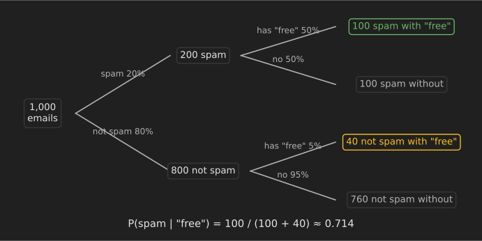
The posterior is the likelihood times the prior, normalized.

Example: 20% of emails are spam. The word "free" appears in 50% of spam and 5% of other mail. Then

$$P(\text{spam} \mid \text{free}) = \frac{0.5 \times 0.2}{0.5 \times 0.2 + 0.05 \times 0.8} = \frac{0.10}{0.14} \approx 0.714$$

7. Naive Bayes classifier

Assume features are conditionally independent given the class:

$$P(y \mid x_1, \dots, x_n) \propto P(y)\prod_{i=1}^n P(x_i \mid y)$$

In data science: a fast, strong baseline for text classification. The independence assumption is usually false, but the ranking of classes is often still right.

Example: Extending concept 6, an email containing both "free" and "winner" multiplies the two likelihood ratios. Work in log space to avoid underflow when there are thousands of words.

8. Counting: permutations and combinations

$$P(n, k) = \frac{n!}{(n - k)!}, \qquad \binom{n}{k} = \frac{n!}{k!\,(n - k)!}$$

Example: There are $\binom{20}{2} = 190$ pairs of features among 20, which is why exhaustive interaction search grows quickly.

9. Random variables

A random variable maps outcomes to numbers. It is discrete if it takes countably many values and continuous if it has a density.

Example: "Number of clicks in a session" is discrete; "time on page" is continuous.

10. PMF, PDF and CDF

A probability mass function gives $P(X = x)$; a density $f$ gives probabilities as areas, $P(a \le X \le b) = \int_a^b f(x)\,dx$; the cumulative distribution function is $F(x) = P(X \le x)$.

In data science: a density value can exceed 1 (it is not a probability). An empirical CDF is often a clearer plot than a histogram because it needs no bin width.

Example: For a uniform density on $[0, 0.5]$, $f(x) = 2$ everywhere in the interval, yet the total area is 1.

Expectation and variance

11. Expected value

$$E[X] = \sum_x x\,P(X = x) \quad\text{or}\quad \int x\,f(x)\,dx$$

Example: A promotion costs $2 per user and returns $50 with probability 5%. The expected profit per user is $0.05 \times 50 - 2 = \$0.50$.

12. Linearity of expectation

$$E[aX + bY] = aE[X] + bE[Y]$$

This holds even when $X$ and $Y$ are dependent.

Example: The expected number of users who click, among 1,000 with click probabilities $p_i$, is $\sum p_i$, whatever the correlations between users.

13. Variance

$$\operatorname{Var}(X) = E\left[(X - \mu)^2\right] = E[X^2] - (E[X])^2$$

Example: A fair die has $E[X] = 3.5$ and $E[X^2] = \tfrac{91}{6}$, so $\operatorname{Var}(X) = \tfrac{91}{6} - 12.25 = \tfrac{35}{12} \approx 2.92$.

14. Standard deviation and scaling

$\sigma = \sqrt{\operatorname{Var}(X)}$ is in the same units as $X$. $\operatorname{Var}(aX + b) = a^2\operatorname{Var}(X)$.

In data science: standardizing features, $z = (x - \mu)/\sigma$, puts them on comparable scales for gradient-based training and distance-based methods such as k-nearest neighbors.

15. Covariance

$$\operatorname{Cov}(X, Y) = E[(X - \mu_X)(Y - \mu_Y)]$$

Example: For $x = (1, 2, 3, 4)$ and $y = (2, 4, 5, 4)$, the sample covariance is $\tfrac{7}{6} \approx 1.17$: positive, so they tend to rise together.

16. Correlation

$$\rho = \frac{\operatorname{Cov}(X, Y)}{\sigma_X\,\sigma_Y} \in [-1, 1]$$

Example: The data in concept 15 has $r \approx 0.72$. Correlation measures linear association only: $y = x^2$ on symmetric data has $r = 0$ despite a perfect relationship. And correlation alone does not establish causation.

17. Covariance matrix

For a random vector $\mathbf{X}$, $\Sigma = E[(\mathbf{X} - \boldsymbol{\mu})(\mathbf{X} - \boldsymbol{\mu})^{T}]$. It is symmetric and positive semidefinite.

In data science: principal component analysis takes the eigenvectors of $\Sigma$; the Mahalanobis distance $\sqrt{(\mathbf{x} - \boldsymbol{\mu})^{T}\Sigma^{-1}(\mathbf{x} - \boldsymbol{\mu})}$ detects outliers that account for correlation.

Example: The data in concept 15 has $\Sigma = \begin{bmatrix} 1.67 & 1.17 \\ 1.17 & 1.58 \end{bmatrix}$.

18. Law of total expectation

$$E[X] = E\big[E[X \mid Y]\big]$$

Example: If average order value is $40 for new customers (30% of orders) and $60 for returning customers, the overall average is $0.3(40) + 0.7(60) = \$54$.

19. Law of total variance

$$\operatorname{Var}(X) = E\big[\operatorname{Var}(X \mid Y)\big] + \operatorname{Var}\big(E[X \mid Y]\big)$$

Total variance splits into variance within groups plus variance between group means.

In data science: this decomposition is the idea behind ANOVA, and behind variance-reduction methods such as stratified sampling and CUPED in A/B testing.

20. Jensen's inequality

For a convex function $\varphi$: $\varphi(E[X]) \le E[\varphi(X)]$. For concave $\log$: $E[\log X] \le \log E[X]$.

In machine learning: it proves that KL divergence is never negative (concept 69) and gives the evidence lower bound used in variational inference (concept 95).

Example: For $X$ equal to 1 or 9 with equal probability, $E[X^2] = 41 \ge (E[X])^2 = 25$.

Probability distributions

21. Bernoulli distribution

One trial with success probability $p$: $E[X] = p$, $\operatorname{Var}(X) = p(1 - p)$.

In machine learning: the output of a binary classifier is the parameter of a Bernoulli distribution, and binary cross-entropy is its negative log-likelihood.

22. Binomial distribution

The number of successes in $n$ independent Bernoulli trials:

$$P(X = k) = \binom{n}{k}p^k(1 - p)^{n - k}, \qquad E[X] = np, \qquad \operatorname{Var}(X) = np(1 - p)$$

Example: With a 20% click rate, the chance that exactly 3 of 10 users click is $\binom{10}{3}(0.2)^3(0.8)^7 \approx 0.201$.

23. Geometric distribution

The number of trials until the first success: $P(X = k) = (1 - p)^{k - 1}p$, $E[X] = 1/p$.

Example: If 10% of leads convert, a salesperson expects to contact 10 leads per sale.

24. Poisson distribution

Counts of rare events in a fixed interval at rate $\lambda$:

$$P(X = k) = \frac{\lambda^ke^{-\lambda}}{k!}, \qquad E[X] = \operatorname{Var}(X) = \lambda$$

Example: A server averages 3 errors per hour. $P(0 \text{ errors}) = e^{-3} \approx 0.050$ and $P(5) \approx 0.101$. If observed counts have variance much larger than the mean (overdispersion), use a negative binomial model instead.

25. Uniform distribution

On $[a, b]$: density $\frac{1}{b - a}$, mean $\frac{a + b}{2}$, variance $\frac{(b - a)^2}{12}$.

In machine learning: random search for hyperparameters often samples uniformly on a log scale, such as a learning rate between $10^{-5}$ and $10^{-1}$.

26. Exponential distribution

Waiting time between Poisson events: $f(x) = \lambda e^{-\lambda x}$, mean $1/\lambda$. It is memoryless: $P(X > s + t \mid X > s) = P(X > t)$.

Example: If support tickets arrive on average every 10 minutes, the chance of waiting more than 5 minutes is $e^{-0.5} \approx 0.61$, no matter how long you have already waited.

27. Normal distribution

$$f(x) = \frac{1}{\sigma\sqrt{2\pi}}\exp\left(-\frac{(x - \mu)^2}{2\sigma^2}\right)$$

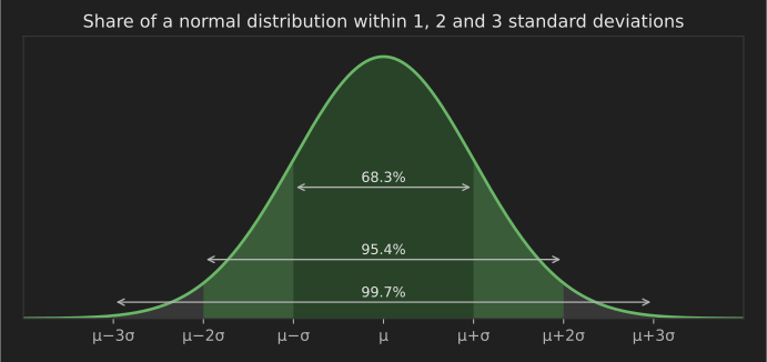
About 68.3%, 95.4% and 99.7% of the probability lies within 1, 2 and 3 standard deviations of the mean.

28. Standard normal and z-scores

$Z = \frac{X - \mu}{\sigma}$ has mean 0 and standard deviation 1, so one table (or scipy.stats.norm) serves every normal distribution.

Example: A model's latency is normal with mean 120 ms and SD 15 ms. A 150 ms request has $z = 2$; only about 2.3% of requests are slower.

29. Multivariate normal distribution

$$f(\mathbf{x}) = \frac{1}{\sqrt{(2\pi)^k\det\Sigma}}\exp\left(-\tfrac{1}{2}(\mathbf{x} - \boldsymbol{\mu})^{T}\Sigma^{-1}(\mathbf{x} - \boldsymbol{\mu})\right)$$

In machine learning: Gaussian mixture models, Gaussian processes, Kalman filters and linear discriminant analysis are all built on it. Its marginals and conditionals are again normal.

30. Log-normal distribution

$X$ is log-normal if $\ln X$ is normal. It is right-skewed and positive.

In data science: incomes, file sizes, session lengths and response times are often roughly log-normal. Model $\log X$, and report medians, which are more stable than means.

31. Beta distribution

A distribution on $[0, 1]$ with density proportional to $p^{\alpha - 1}(1 - p)^{\beta - 1}$ and mean $\frac{\alpha}{\alpha + \beta}$.

In machine learning: the natural prior for a probability, such as a click-through rate. Thompson sampling for multi-armed bandits draws from a Beta posterior for each arm.

32. Gamma distribution

Positive and right-skewed, with shape $k$ and scale $\theta$: mean $k\theta$, variance $k\theta^2$. The exponential and chi-square distributions are special cases.

In machine learning: the conjugate prior for a Poisson rate or a normal precision.

33. Categorical and multinomial distributions

The categorical distribution picks one of $K$ classes with probabilities $p_1, \dots, p_K$; the multinomial counts outcomes over $n$ such draws.

In machine learning: a softmax output layer (concept 76) parameterizes a categorical distribution; a language model's next-token prediction is one.

34. Dirichlet distribution

A distribution over probability vectors $(p_1, \dots, p_K)$ with $\sum p_i = 1$; the multivariate version of the Beta.

In machine learning: latent Dirichlet allocation (LDA) uses it for topic proportions in documents.

35. Student's t distribution

The distribution of $\frac{\bar{X} - \mu}{s / \sqrt{n}}$ for normal data. It has heavier tails than the normal and approaches it as degrees of freedom grow.

Example: With 15 degrees of freedom the two-sided 95% critical value is 2.131, against 1.960 for the normal. Small samples need wider intervals.

36. Chi-square distribution

The sum of $k$ squared independent standard normals. It describes sample variances and the test statistics in goodness-of-fit and independence tests (concept 60).

Limit theorems and sampling

37. Law of large numbers

The sample mean $\bar{X}_n$ converges to $\mu$ as $n \to \infty$.

In data science: why averages over more data are more reliable, and why a small A/B test can show a large "effect" that disappears with more traffic.

38. Central limit theorem

For i.i.d. data with finite variance, $\frac{\bar{X}_n - \mu}{\sigma / \sqrt{n}}$ approaches a standard normal distribution as $n$ grows, whatever the shape of the original distribution.

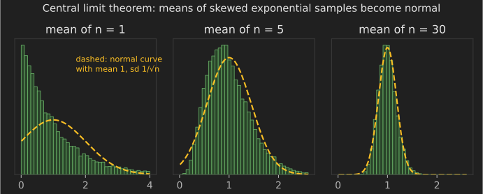
In data science: it justifies normal-based confidence intervals and tests for means and proportions, even for skewed metrics such as revenue, provided samples are large enough. Very heavy tails need much larger samples.

39. Standard error

$$\operatorname{SE}(\bar{X}) = \frac{\sigma}{\sqrt{n}}$$

Example: With $\sigma = 15$ and $n = 100$, $\operatorname{SE} = 1.5$. To halve the standard error you need four times as much data.

40. Bootstrap

Estimate the sampling distribution of any statistic by resampling the data with replacement many times and recomputing the statistic.

In data science: confidence intervals for medians, ratios, AUC and other metrics with no simple formula. It assumes the sample represents the population and needs care with dependent data, such as several sessions per user (resample users, not sessions).

41. Monte Carlo estimation

Approximate an expectation by averaging random draws: $E[g(X)] \approx \frac{1}{N}\sum g(x_i)$. The error shrinks like $1/\sqrt{N}$.

Example: Estimating $\pi$ as 4 times the fraction of random points in the unit square that fall inside the quarter circle: with $10^6$ points the standard error is about 0.0016.

42. Markov and Chebyshev inequalities

$$P(X \ge a) \le \frac{E[X]}{a} \;(X \ge 0), \qquad P(|X - \mu| \ge k\sigma) \le \frac{1}{k^2}$$

Example: For any distribution with finite variance, at most 25% of values lie more than 2 standard deviations from the mean. The normal distribution gives 4.6%; Chebyshev is the worst case.

43. Hoeffding's inequality

For the mean of $n$ independent values bounded in $[0, 1]$:

$$P(|\bar{X} - \mu| \ge \varepsilon) \le 2e^{-2n\varepsilon^2}$$

In machine learning: the basis of many generalization bounds and of sample-size guarantees.

Example: To estimate an accuracy within $\pm 0.05$ with 95% confidence, $n \ge \frac{\ln(2/0.05)}{2(0.05)^2} \approx 738$ test examples suffice for any model.

44. Sampling bias

A sample is biased when the selection process makes some units more likely to be included in a way related to the outcome. More data does not fix it.

In data science: survivorship bias (analyzing only customers who stayed), selection bias (training a credit model only on approved applicants) and non-response bias all produce models that fail on the real population.

Estimation

45. Estimators and bias

An estimator $\hat{\theta}$ is a function of the data. Its bias is $E[\hat{\theta}] - \theta$.

Example: The sample variance with divisor $n$ is biased low by a factor $\frac{n - 1}{n}$; dividing by $n - 1$ (Bessel's correction) removes the bias.

46. Mean squared error and the bias–variance decomposition

$$\operatorname{MSE}(\hat{\theta}) = \operatorname{Bias}(\hat{\theta})^2 + \operatorname{Var}(\hat{\theta})$$

In machine learning: a slightly biased estimator with much lower variance often wins. Regularization (concept 77) and shrinkage deliberately add bias to cut variance.

47. Maximum likelihood estimation

Choose the parameters that make the observed data most probable:

$$\hat{\theta}_{\text{MLE}} = \arg\max_\theta\sum_{i=1}^n\log p(x_i \mid \theta)$$

In machine learning: minimizing cross-entropy or mean squared error is maximum likelihood under a Bernoulli/categorical or Gaussian noise model.

48. MLE examples

For Bernoulli data, $\hat{p} = \frac{\text{successes}}{n}$. For normal data, $\hat{\mu} = \bar{x}$ and $\hat{\sigma}^2 = \frac{1}{n}\sum(x_i - \bar{x})^2$ (the biased version from concept 45).

Example: 7 conversions out of 10 trials give $\hat{p} = 0.7$.

49. Maximum a posteriori (MAP) estimation

$$\hat{\theta}_{\text{MAP}} = \arg\max_\theta\left[\log p(\text{data} \mid \theta) + \log p(\theta)\right]$$

The prior acts as a penalty term; with a flat prior, MAP equals MLE.

50. Conjugate priors: Beta–binomial

With a $\operatorname{Beta}(\alpha, \beta)$ prior and $s$ successes in $n$ trials, the posterior is $\operatorname{Beta}(\alpha + s, \beta + n - s)$.

Example: A uniform $\operatorname{Beta}(1, 1)$ prior and 7 conversions in 10 trials give $\operatorname{Beta}(8, 4)$, with posterior mean $\tfrac{8}{12} \approx 0.667$. That is pulled slightly toward 0.5 compared with the MLE of 0.7, which protects against over-reading 10 data points.

51. Credible intervals

A 95% credible interval contains the parameter with 95% posterior probability.

Example: For the $\operatorname{Beta}(8, 4)$ posterior above, the central 95% credible interval is about $(0.39, 0.89)$: ten trials say very little.

52. Fisher information and the Cramér–Rao bound

$I(\theta) = -E\left[\frac{\partial^2}{\partial\theta^2}\log p(X \mid \theta)\right]$, and any unbiased estimator from $n$ i.i.d. observations has $\operatorname{Var}(\hat{\theta}) \ge \frac{1}{nI(\theta)}$.

Example: For Bernoulli data $I(p) = \frac{1}{p(1 - p)}$, so no unbiased estimator beats variance $\frac{p(1 - p)}{n}$. The sample proportion achieves it.

53. Method of moments

Set sample moments equal to theoretical moments and solve for the parameters.

Example: For a uniform distribution on $[0, \theta]$, $E[X] = \theta/2$, so $\hat{\theta} = 2\bar{x}$. It is simple, but here the MLE ($\max x_i$) has much lower mean squared error.

54. Consistency

An estimator is consistent if it converges to the true value as $n \to \infty$.

In machine learning: an estimator can be consistent yet badly biased in small samples, and a model trained on biased data (concept 44) can converge confidently to the wrong answer.

Statistical inference and experiments

55. Confidence intervals

A 95% confidence interval comes from a procedure that captures the true parameter in 95% of repeated samples. It is not a 95% probability statement about one computed interval.

Example: 520 of 1,000 surveyed users prefer a design: $0.52 \pm 1.96\sqrt{\frac{0.52 \times 0.48}{1000}} = 0.52 \pm 0.031$.

56. Hypothesis testing

State a null hypothesis $H_0$ (no effect) and an alternative, compute a test statistic, and reject $H_0$ if data this extreme would be unlikely under it.

In data science: the logic behind A/B tests, feature-significance checks and drift detection.

57. p-values

The probability, assuming $H_0$ is true, of a result at least as extreme as the one observed. It is not the probability that $H_0$ is true, and it says nothing about the size of the effect.

Example: A sample of 16 with mean 52 and SD 8, tested against $\mu = 50$: $t = \frac{2}{8/4} = 1.0$ with 15 degrees of freedom gives a two-sided $p \approx 0.33$. The data are consistent with no difference.

58. Type I and type II errors, and power

A type I error rejects a true $H_0$ (rate $\alpha$); a type II error misses a real effect (rate $\beta$). Power, $1 - \beta$, is the chance of detecting an effect of a given size.

In data science: underpowered experiments miss real improvements, and the ones that do reach significance tend to overstate the effect.

59. t-tests

Compare a mean with a value (one-sample), two group means (Welch's two-sample test, which does not assume equal variances), or paired measurements.

Example: Comparing a model's error on the same 50 test sets before and after a change calls for a paired test, which removes the variation between test sets.

60. Chi-square test of independence

$$\chi^2 = \sum\frac{(O - E)^2}{E}$$

Example: For the table $\begin{bmatrix} 30 & 20 \\ 20 & 30 \end{bmatrix}$ (variant by converted or not), each expected count is 25, so $\chi^2 = 4 \times \frac{25}{25} = 4.0$ with 1 degree of freedom, giving $p \approx 0.046$.

61. A/B testing

Randomly assign units to control and treatment, fix the sample size and metric in advance, then compare. Randomization is what lets you read a difference as caused by the change.

In data science: check for sample-ratio mismatch (unequal group sizes signal a bug), and do not stop the moment $p < 0.05$; repeated peeking inflates false positives unless you use a sequential testing method.

62. Sample size calculation

For comparing two proportions $p_1$ and $p_2$ with significance $\alpha$ and power $1 - \beta$:

$$n \approx \frac{(z_{1-\alpha/2} + z_{1-\beta})^2\left[p_1(1 - p_1) + p_2(1 - p_2)\right]}{(p_1 - p_2)^2} \text{ per group}$$

Example: Detecting a lift from 10% to 12% with $\alpha = 0.05$ and 80% power needs about 3,840 users per group. Halving the detectable lift roughly quadruples the sample.

63. Multiple comparisons

Run 20 independent tests at $\alpha = 0.05$ with no real effects, and the chance of at least one false positive is $1 - 0.95^{20} \approx 64\%$.

Fixes: the Bonferroni correction tests each at $\alpha / m$ (here 0.0025); the Benjamini–Hochberg procedure controls the false discovery rate and keeps more power when many hypotheses are tested.

64. Permutation tests

Shuffle the group labels many times and recompute the statistic to build its null distribution directly. They need no distributional assumptions beyond exchangeability under $H_0$.

Example: To test whether a feature's importance score is meaningful, permute that feature's values and see how often a score as high appears by chance.

65. Effect size

A standardized magnitude, independent of sample size. Cohen's $d = \frac{\bar{x}_1 - \bar{x}_2}{s_{\text{pooled}}}$.

In data science: with millions of users, trivially small effects become "significant". Always report the effect with a confidence interval, not just a p-value.

66. Bayesian A/B testing

Model each variant's rate with a posterior (concept 50) and report $P(\text{B better than A})$ and the expected loss of choosing each.

Example: With $\operatorname{Beta}(1 + s_A, 1 + n_A - s_A)$ and the same for B, draw 100,000 samples from each and count how often B's draw is larger. The answer is directly interpretable, but it still depends on the prior and still suffers if you stop early on noise.

Information theory

67. Entropy

$$H(X) = -\sum_x p(x)\log_2 p(x)$$

The average surprise, in bits.

Example: A fair coin has 1 bit of entropy; a coin with $P(H) = 0.9$ has about 0.469 bits. Decision trees choose splits that reduce entropy the most (information gain).

68. Cross-entropy

$$H(p, q) = -\sum_x p(x)\log q(x)$$

In machine learning: the standard classification loss. For one example whose true class gets predicted probability $q$, the loss is $-\ln q$: 0.223 when $q = 0.8$ but 2.303 when $q = 0.1$. Confident mistakes are punished heavily.

69. KL divergence

$$D_{\text{KL}}(p \,\Vert\, q) = \sum_x p(x)\log\frac{p(x)}{q(x)} \ge 0$$

It is zero only when $p = q$, and it is not symmetric.

Example: From a fair coin $p$ to a model $q$ with $P(H) = 0.9$: $0.5\ln\frac{0.5}{0.9} + 0.5\ln\frac{0.5}{0.1} \approx 0.511$ nats. KL appears in variational autoencoders, knowledge distillation and the penalty that keeps a fine-tuned language model close to its reference model.

70. Mutual information

$$I(X; Y) = D_{\text{KL}}\big(p(x, y) \,\Vert\, p(x)p(y)\big)$$

The reduction in uncertainty about $X$ from knowing $Y$. Unlike correlation, it detects nonlinear dependence.

In data science: feature selection (mutual_info_classif in scikit-learn) and contrastive representation learning.

71. Log loss is negative log-likelihood

Minimizing average cross-entropy over a dataset is exactly maximizing the likelihood of the labels under the model (concept 47). This is why "cross-entropy loss" and "negative log-likelihood loss" are the same thing in most libraries.

72. Perplexity

$$\text{perplexity} = \exp(\text{average cross-entropy in nats})$$

Example: A language model with average cross-entropy 2.0 nats per token has perplexity $e^2 \approx 7.39$: on average it is as uncertain as a uniform choice among about 7.4 tokens.

Regression and modeling

73. Linear regression as maximum likelihood

If $y = \mathbf{x}^{T}\boldsymbol{\beta} + \varepsilon$ with $\varepsilon \sim N(0, \sigma^2)$, maximizing the likelihood is the same as minimizing the sum of squared errors, giving $\hat{\boldsymbol{\beta}} = (X^{T}X)^{-1}X^{T}\mathbf{y}$.

Example: See the worked fit in 101 linear algebra problems with solutions, problem 95.

74. Coefficient of determination (R²)

$$R^2 = 1 - \frac{\sum(y_i - \hat{y}_i)^2}{\sum(y_i - \bar{y})^2}$$

The share of variance explained. It never falls when you add features, so compare models on held-out data or with adjusted $R^2$.

75. Logistic regression

$$P(y = 1 \mid \mathbf{x}) = \sigma(\mathbf{w}^{T}\mathbf{x} + b), \qquad \sigma(z) = \frac{1}{1 + e^{-z}}$$

Each coefficient changes the log-odds $\ln\frac{p}{1 - p}$ linearly.

Example: A coefficient of 0.693 doubles the odds per unit increase in that feature, because $e^{0.693} \approx 2$.

76. Softmax

$$\operatorname{softmax}(\mathbf{z})_k = \frac{e^{z_k}}{\sum_j e^{z_j}}$$

Example: Scores $(2, 1, 0)$ become probabilities $(0.665, 0.245, 0.090)$. Subtracting the largest score before exponentiating gives the same result without overflow.

77. Regularization as a prior

L2 regularization (ridge) is MAP estimation with a Gaussian prior on the weights; L1 (lasso) corresponds to a Laplace prior, which pushes some weights exactly to zero.

In machine learning: weight decay in neural networks is the L2 version; the regularization strength plays the role of the prior's precision.

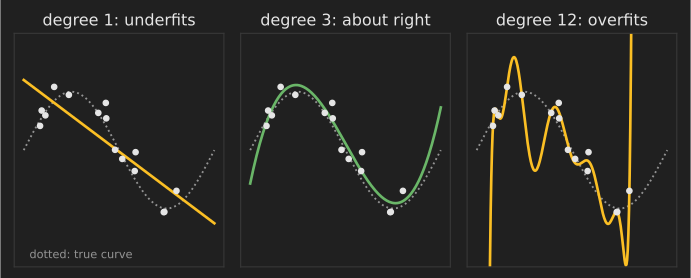
78. Bias–variance tradeoff

Expected test error = bias² + variance + irreducible noise. Simple models underfit (high bias); flexible models overfit (high variance).

79. Cross-validation

Split data into $k$ folds, train on $k - 1$, validate on the remaining one, and average. It estimates generalization error and guides model choice.

In data science: split by group (user, patient) or by time when examples are related, or the estimate will be optimistic. Any preprocessing fitted on the data, such as scaling or imputation, must be fitted inside each fold to avoid leakage.

80. Overfitting and data leakage

Overfitting is learning noise in the training data. Leakage is letting information unavailable at prediction time into training, such as a "days since cancellation" feature in a churn model. Leakage produces excellent validation scores and a model that fails in production.

81. Generalized linear models

A GLM links a linear predictor to the mean of a distribution from the exponential family: identity link with normal errors (linear regression), logit link with Bernoulli (logistic), log link with Poisson (count regression).

Example: Model website visits per day with Poisson regression so predictions stay positive and variance grows with the mean.

82. Residual diagnostics

Plot residuals against fitted values and check for patterns, changing spread (heteroscedasticity) and outliers.

In data science: a funnel-shaped residual plot means standard errors from ordinary least squares are wrong; use robust standard errors or transform the target.

Evaluating classifiers and predictions

83. Confusion matrix

Counts of true positives (TP), false positives (FP), false negatives (FN) and true negatives (TN) at a chosen threshold.

Example: TP = 80, FP = 20, FN = 40, TN = 860. Accuracy is $\tfrac{940}{1000} = 94\%$, which sounds good but hides that a third of positives are missed.

84. Precision and recall

$$\text{precision} = \frac{TP}{TP + FP}, \qquad \text{recall} = \frac{TP}{TP + FN}$$

Example: For concept 83, precision is $\tfrac{80}{100} = 0.80$ and recall is $\tfrac{80}{120} \approx 0.67$.

85. F1 score

$$F_1 = \frac{2 \cdot \text{precision} \cdot \text{recall}}{\text{precision} + \text{recall}}$$

Example: $\frac{2(0.8)(0.667)}{0.8 + 0.667} \approx 0.727$. The harmonic mean punishes imbalance between the two. Use $F_\beta$ when recall matters $\beta$ times as much as precision.

86. ROC curve and AUC

The ROC curve plots true positive rate against false positive rate across all thresholds. The area under it (AUC) is the probability that a random positive scores higher than a random negative.

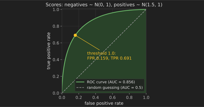
87. Precision–recall curves for imbalanced data

When positives are rare, ROC curves can look good while precision is poor, because the false positive rate divides by a huge number of negatives. Precision–recall curves and average precision show the trade-off that matters for rare-event detection such as fraud.

88. The base-rate fallacy

A test that is 95% sensitive and 95% specific, applied where only 1% have the condition, gives a positive predictive value of

$$\frac{0.95 \times 0.01}{0.95 \times 0.01 + 0.05 \times 0.99} \approx 0.16$$

In machine learning: a fraud model's alerts are mostly false alarms when fraud is rare, even if the model is accurate. This is Bayes' theorem (concept 6) again.

89. Calibration and the Brier score

A model is calibrated if, among predictions of 70%, about 70% are positive. The Brier score $\frac{1}{n}\sum(p_i - y_i)^2$ rewards both calibration and sharpness.

In data science: boosted trees and deep networks are often miscalibrated; Platt scaling and isotonic regression fix this after training. Calibration matters whenever probabilities feed decisions, such as expected cost.

90. Choosing a decision threshold

The best threshold depends on costs, not on 0.5. If a false negative costs 10 times a false positive and probabilities are calibrated, predict positive when $p > \frac{1}{1 + 10} \approx 0.09$.

91. MAE versus RMSE

$$\text{MAE} = \frac{1}{n}\sum|e_i|, \qquad \text{RMSE} = \sqrt{\frac{1}{n}\sum e_i^2}$$

Example: Errors $(1, 1, 1, 1, 6)$ give MAE = 2 but RMSE = $\sqrt{8} \approx 2.83$; RMSE weights the one large error heavily. Minimizing MAE targets the conditional median; minimizing squared error targets the mean.

92. Quantiles and prediction intervals

Instead of a single prediction, estimate quantiles (with pinball loss) to give a range, such as a 10th–90th percentile delivery time.

In data science: conformal prediction wraps any model to produce intervals with a guaranteed coverage rate on exchangeable data.

Probabilistic machinery in modern machine learning

93. Markov chains

A process where the next state depends only on the current one. A well-behaved chain converges to a stationary distribution $\pi$ with $\pi P = \pi$.

Example: Google's original PageRank is the stationary distribution of a random surfer on the web graph.

94. Markov chain Monte Carlo

Build a Markov chain whose stationary distribution is the posterior you want, then sample from it. The Metropolis–Hastings rule accepts a proposed move from $\theta$ to $\theta'$ with probability $\min\left(1, \frac{p(\theta')q(\theta \mid \theta')}{p(\theta)q(\theta' \mid \theta)}\right)$, which only needs the posterior up to a constant.

In data science: probabilistic programming tools such as Stan and PyMC use advanced versions (Hamiltonian Monte Carlo, NUTS).

95. Variational inference and the ELBO

Approximate an intractable posterior $p(z \mid x)$ with a simpler $q(z)$ by maximizing the evidence lower bound:

$$\log p(x) = \underbrace{E_q[\log p(x, z) - \log q(z)]}_{\text{ELBO}} + D_{\text{KL}}\big(q(z) \,\Vert\, p(z \mid x)\big)$$

Since the KL term is non-negative, the ELBO is a lower bound on $\log p(x)$.

In machine learning: variational autoencoders and scalable Bayesian models train by maximizing it.

96. The reparameterization trick

Write $z = \mu + \sigma\varepsilon$ with $\varepsilon \sim N(0, 1)$, so a random sample becomes a differentiable function of $\mu$ and $\sigma$ and gradients can flow through it. This is what makes variational autoencoders trainable by backpropagation.

97. Expectation–maximization and Gaussian mixtures

For models with hidden variables, alternate an E-step (compute each point's probability of belonging to each component) and an M-step (refit parameters with those weights). Each iteration never decreases the likelihood.

Example: Fitting a two-component Gaussian mixture to customer spending finds a "casual" and a "power user" cluster with soft memberships, unlike k-means' hard assignments.

98. Kernel density estimation

$$\hat{f}(x) = \frac{1}{nh}\sum_{i=1}^n K\left(\frac{x - x_i}{h}\right)$$

A smooth, non-parametric density estimate. The bandwidth $h$ matters far more than the kernel shape; Silverman's rule of thumb is $h \approx 1.06\,\hat{\sigma}\,n^{-1/5}$ for roughly normal data.

99. Gaussian processes

A distribution over functions in which any finite set of values is multivariate normal, defined by a mean and a kernel such as $k(x, x') = \exp\left(-\frac{(x - x')^2}{2\ell^2}\right)$.

In machine learning: Gaussian processes give predictions with uncertainty from small data and power Bayesian optimization for hyperparameter tuning.

100. Simpson's paradox

A trend in every subgroup can reverse when the groups are combined, because the groups differ in size and composition.

In data science: always check whether an aggregate comparison is confounded by mix (device, region, user tenure). The companion article works through the 1973 Berkeley admissions data as an example.

101. Correlation, causation and confounding

A confounder affects both the treatment and the outcome, creating association without causation. Randomized experiments break confounding; without them, methods such as matching, instrumental variables, difference-in-differences and causal graphs try to recover causal effects under stated assumptions.

Example: Users who use a feature churn less, but engaged users are both more likely to find the feature and less likely to churn. Only an experiment, or a credible causal design, tells you whether promoting the feature would reduce churn.

Common mistakes

• Reading a p-value as the probability the null is true (concept 57), or treating "not significant" as "no effect".
• Ignoring base rates: high accuracy on rare events can still mean most alerts are false (concept 88).
• Reporting accuracy on imbalanced data instead of precision, recall and PR curves (concepts 84–87).
• Peeking at an A/B test and stopping when it looks good, and testing many metrics without correction (concepts 61 and 63).
• Leaking information through preprocessing fitted on all the data, or random splits of grouped or time-ordered data (concepts 79 and 80).
• Assuming independence when the same users, sessions or time periods appear many times (concept 4).
• Confusing correlation with causation (concept 101).

Next steps

• Work through 100 applied problems in probability and statistics examples for real-world applications.
• See how loss functions are minimized in 100 mathematical optimization techniques used in AI, engineering and research.
• Review the linear algebra behind covariance matrices and PCA in 101 linear algebra concepts for machine learning.
• Brush up on integrals and series in 100 calculus formulas, theorems and examples, and browse the mathematics category.

References

• All of Statistics: A Concise Course in Statistical Inference, Larry Wasserman, Springer (2004).
• An Introduction to Statistical Learning, Gareth James, Daniela Witten, Trevor Hastie, Robert Tibshirani and Jonathan Taylor, Springer (2nd edition, 2021; Python edition, 2023). https://www.statlearning.com/
• Pattern Recognition and Machine Learning, Christopher M. Bishop, Springer (2006). https://www.microsoft.com/en-us/research/people/cmbishop/prml-book/
• Deep Learning, Ian Goodfellow, Yoshua Bengio and Aaron Courville, MIT Press (2016), chapter 3, "Probability and Information Theory". https://www.deeplearningbook.org/contents/prob.html
• Introductory Statistics 2e, Barbara Illowsky and Susan Dean, OpenStax (2023). https://openstax.org/details/books/introductory-statistics-2e
• NIST/SEMATECH e-Handbook of Statistical Methods, National Institute of Standards and Technology. https://www.itl.nist.gov/div898/handbook/
• Benjamini, Y. and Hochberg, Y. (1995). "Controlling the false discovery rate: a practical and powerful approach to multiple testing." Journal of the Royal Statistical Society, Series B, 57(1), 289–300. https://doi.org/10.1111/j.2517-6161.1995.tb02031.x
• Kingma, D. P. and Welling, M. (2013). "Auto-Encoding Variational Bayes." arXiv:1312.6114. https://arxiv.org/abs/1312.6114
• Kohavi, R., Tang, D. and Xu, Y. (2020). Trustworthy Online Controlled Experiments: A Practical Guide to A/B Testing. Cambridge University Press.