100 Best Calculus Formulas, Theorems, and Examples Every Student Should Know

Calculus is the mathematics of change and accumulation. Derivatives measure how fast something changes; integrals add up small pieces into a whole; and the fundamental theorem of calculus says these two operations undo each other. Almost everything else in a calculus course, from optimization to series to differential equations, is built from those ideas.

This article collects 100 formulas and theorems that a student meets across single-variable calculus, series, multivariable calculus, vector calculus and a first look at differential equations. For each one you get the statement, the conditions under which it holds (theorems are only as good as their hypotheses), and a short worked example. Every example was recomputed with SymPy before publication.

The basic differentiation and integration rules also appear, more briefly, in 100 mathematics formulas every student should know. This article goes further: it states the theorems behind the rules and covers series, several variables and vector fields. All angles are in radians.

Limits and continuity

1. The epsilon–delta definition of a limit

$$\lim_{x \to a} f(x) = L \iff \forall \varepsilon > 0\; \exists \delta > 0 : 0 < |x - a| < \delta \Rightarrow |f(x) - L| < \varepsilon$$

Example: To show $\lim_{x \to 2}(3x + 1) = 7$: $|3x + 1 - 7| = 3|x - 2|$, so choosing $\delta = \varepsilon / 3$ guarantees $|f(x) - 7| < \varepsilon$.

2. Limit laws

Limits of sums, differences, products and quotients are the sums, differences, products and quotients of the limits, provided each limit exists and no denominator limit is zero.

Example: $\lim_{x \to 2}(x^2 + 3x) = 4 + 6 = 10$.

3. Squeeze theorem

If $g(x) \le f(x) \le h(x)$ near $a$ and $\lim g = \lim h = L$, then $\lim f = L$.

Example: $-x^2 \le x^2\sin(1/x) \le x^2$, and both bounds go to 0, so $\lim_{x \to 0} x^2\sin(1/x) = 0$ even though $\sin(1/x)$ oscillates wildly.

4. Limits at infinity of rational functions

Divide numerator and denominator by the highest power of $x$ in the denominator.

Example: $\displaystyle\lim_{x \to \infty}\frac{3x^2 + 1}{5x^2 - x} = \lim_{x \to \infty}\frac{3 + 1/x^2}{5 - 1/x} = \frac{3}{5}$.

5. The limit that defines e

$$\lim_{n \to \infty}\left(1 + \frac{1}{n}\right)^n = e \approx 2.71828$$

Example: Compounding 100% interest $n$ times a year turns $1 into $(1 + 1/n)^n$ dollars; as $n \to \infty$ (continuous compounding) the amount approaches $2.72.

6. Exponential and logarithm limits

$$\lim_{x \to 0}\frac{e^x - 1}{x} = 1, \qquad \lim_{x \to 0}\frac{\ln(1 + x)}{x} = 1$$

Example: $\displaystyle\lim_{x \to 0}\frac{e^{3x} - 1}{x} = 3 \cdot \lim_{x \to 0}\frac{e^{3x} - 1}{3x} = 3$.

7. One-sided limits

$\lim_{x \to a} f(x)$ exists exactly when both one-sided limits exist and are equal.

Example: For $f(x) = |x|/x$, the left limit at 0 is $-1$ and the right limit is $1$, so the two-sided limit does not exist.

8. Continuity and removable discontinuities

$f$ is continuous at $a$ when $\lim_{x \to a} f(x) = f(a)$.

Example: $f(x) = \dfrac{x^2 - 1}{x - 1}$ is undefined at 1, but equals $x + 1$ elsewhere, so the limit is 2. Defining $f(1) = 2$ removes the discontinuity.

9. Intermediate value theorem

If $f$ is continuous on $[a, b]$ and $N$ lies between $f(a)$ and $f(b)$, then $f(c) = N$ for some $c$ in $(a, b)$.

Example: $f(x) = x^3 + x - 1$ has $f(0) = -1$ and $f(1) = 1$, so it has a root between 0 and 1. Bisection, the simplest root-finding algorithm, is this theorem applied repeatedly.

10. Extreme value theorem

A function continuous on a closed, bounded interval $[a, b]$ attains a maximum and a minimum there.

Example: $f(x) = x^2$ on $[-1, 2]$ attains its maximum 4 at $x = 2$ and minimum 0 at $x = 0$. On the open interval $(0, 1)$, $f(x) = 1/x$ has no maximum: the hypothesis "closed" matters.

11. L'Hôpital's rule for 0/0

If $f(a) = g(a) = 0$ and $f, g$ are differentiable near $a$ with $g'(x) \ne 0$, then $\lim \frac{f}{g} = \lim \frac{f'}{g'}$ when the right side exists.

Example: $\displaystyle\lim_{x \to 0}\frac{1 - \cos x}{x^2} = \lim_{x \to 0}\frac{\sin x}{2x} = \frac{1}{2}$.

12. The indeterminate form 1^∞

Take logarithms, find the limit of the logarithm, then exponentiate.

Example: $\displaystyle\lim_{x \to \infty}\left(1 + \frac{2}{x}\right)^x$: the log is $x\ln(1 + 2/x) \to 2$, so the limit is $e^2$.

Derivatives

13. Definition of the derivative

$$f'(x) = \lim_{h \to 0}\frac{f(x + h) - f(x)}{h}$$

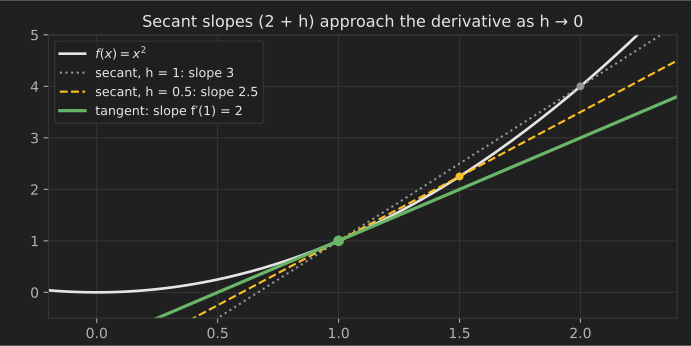
Example: For $f(x) = x^2$ at $x = 1$, the difference quotient is $\frac{(1 + h)^2 - 1}{h} = 2 + h \to 2$.

14. Differentiable implies continuous

If $f'(a)$ exists, $f$ is continuous at $a$. The converse is false.

Example: $|x|$ is continuous at 0 but not differentiable there: the difference quotient is $-1$ from the left and $+1$ from the right.

15. Power, constant multiple and sum rules

$$\frac{d}{dx}\left(a x^n + b x^m\right) = a n x^{n-1} + b m x^{m-1}$$

Example: $\frac{d}{dx}(4x^3 - 5x + 7) = 12x^2 - 5$.

16. Product rule

$$(fg)' = f'g + fg'$$

Example: $\frac{d}{dx}(x^2e^x) = 2xe^x + x^2e^x = e^x(x^2 + 2x)$.

17. Quotient rule

$$\left(\frac{f}{g}\right)' = \frac{f'g - fg'}{g^2}$$

Example: $\dfrac{d}{dx}\dfrac{x}{x^2 + 1} = \dfrac{(x^2 + 1) - x(2x)}{(x^2 + 1)^2} = \dfrac{1 - x^2}{(x^2 + 1)^2}$.

18. Chain rule

$$\frac{d}{dx}f(g(x)) = f'(g(x))\,g'(x)$$

Example: $\frac{d}{dx}\sin(x^2) = \cos(x^2) \cdot 2x$.

19. Derivatives of tangent, secant, cotangent and cosecant

$$(\tan x)' = \sec^2 x, \quad (\sec x)' = \sec x\tan x, \quad (\cot x)' = -\csc^2 x, \quad (\csc x)' = -\csc x\cot x$$

Example: $\frac{d}{dx}\tan(3x) = 3\sec^2(3x)$.

20. Derivatives of inverse trigonometric functions

$$(\arcsin x)' = \frac{1}{\sqrt{1 - x^2}}, \qquad (\arctan x)' = \frac{1}{1 + x^2}$$

Example: The slope of $\arctan x$ at $x = 1$ is $\tfrac{1}{2}$.

21. Exponentials and logarithms in any base

$$\frac{d}{dx}a^x = a^x\ln a, \qquad \frac{d}{dx}\log_a x = \frac{1}{x\ln a}$$

Example: $\frac{d}{dx}2^x = 2^x\ln 2 \approx 0.693 \cdot 2^x$. So a quantity that doubles every unit of time is, at each instant, growing at about 69% of its current size per unit of time.

22. Implicit differentiation

Differentiate both sides with respect to $x$, treating $y$ as a function of $x$.

Example: For the circle $x^2 + y^2 = 25$, $2x + 2yy' = 0$, so $y' = -x/y$. At $(3, 4)$ the slope is $-\tfrac{3}{4}$.

23. Logarithmic differentiation

For products, quotients and variable exponents, differentiate $\ln y$ instead of $y$.

Example: $y = x^x$: $\ln y = x\ln x$, so $\frac{y'}{y} = \ln x + 1$ and $y' = x^x(\ln x + 1)$.

24. Derivative of an inverse function

$$(f^{-1})'(b) = \frac{1}{f'(a)} \quad\text{where } f(a) = b$$

Example: $f(x) = x^3 + x$ has $f(1) = 2$ and $f'(1) = 4$, so $(f^{-1})'(2) = \tfrac{1}{4}$, without ever solving for $f^{-1}$.

25. Higher derivatives

$f''$ is the derivative of $f'$, and so on. For position $s(t)$, $s'$ is velocity and $s''$ is acceleration.

Example: $\frac{d^n}{dx^n}e^{2x} = 2^ne^{2x}$.

26. Hyperbolic functions

$$\sinh x = \frac{e^x - e^{-x}}{2}, \quad \cosh x = \frac{e^x + e^{-x}}{2}, \quad (\sinh x)' = \cosh x, \quad (\cosh x)' = \sinh x$$

Example: A hanging chain or cable under its own weight takes the shape $y = a\cosh(x/a)$, the catenary.

27. Linear approximation

$$f(x) \approx f(a) + f'(a)(x - a) \quad\text{for } x \text{ near } a$$

Example: With $f(x) = \sqrt{x}$ and $a = 4$: $\sqrt{4.1} \approx 2 + \frac{0.1}{4} = 2.025$. The true value is $2.02485$.

28. Differentials and error propagation

$$dy = f'(x)\,dx$$

Example: A sphere's radius is measured as $10 \pm 0.1$ cm. Since $V = \frac{4}{3}\pi r^3$, $dV = 4\pi r^2\,dr = 4\pi(100)(0.1) \approx 125.7\ \text{cm}^3$, about 3% of the volume, three times the 1% error in $r$.

29. Related rates

Differentiate an equation linking the quantities with respect to time.

Example: A 10 ft ladder slides down a wall. When the base is 6 ft out and moving away at 2 ft/s, $x^2 + y^2 = 100$ gives $x\dot{x} + y\dot{y} = 0$. With $y = 8$: $\dot{y} = -\frac{6 \cdot 2}{8} = -1.5$ ft/s. The top is falling at 1.5 ft/s.

30. Newton's method

$$x_{n+1} = x_n - \frac{f(x_n)}{f'(x_n)}$$

Example: For $\sqrt{2}$, use $f(x) = x^2 - 2$ and $x_0 = 1$: $x_1 = 1.5$, $x_2 = 1.41667$, $x_3 = 1.414216$. The number of correct digits roughly doubles each step.

31. Mean value theorem

If $f$ is continuous on $[a, b]$ and differentiable on $(a, b)$, some $c$ in $(a, b)$ satisfies

$$f'(c) = \frac{f(b) - f(a)}{b - a}$$

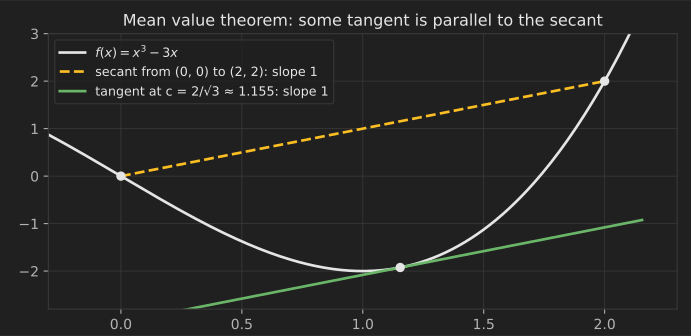
Example: $f(x) = x^3 - 3x$ on $[0, 2]$ has average slope $\frac{2 - 0}{2} = 1$. Solving $3c^2 - 3 = 1$ gives $c = 2/\sqrt{3} \approx 1.155$. If a car's average speed over a trip is 60 km/h, the speedometer read exactly 60 at some instant.

32. Rolle's theorem

The special case of the mean value theorem with $f(a) = f(b)$: then $f'(c) = 0$ for some $c$ in $(a, b)$.

Example: $f(x) = x^2 - 4x$ has $f(0) = f(4) = 0$, and $f'(c) = 2c - 4 = 0$ at $c = 2$.

Applications of derivatives

33. Critical points and the first derivative test

Critical points are where $f' = 0$ or $f'$ is undefined. If $f'$ changes from $+$ to $-$, there is a local maximum; from $-$ to $+$, a local minimum.

Example: $f(x) = x^3 - 3x$ has $f'(x) = 3(x - 1)(x + 1)$. It has a local maximum $f(-1) = 2$ and a local minimum $f(1) = -2$.

34. Concavity and the second derivative test

$f'' > 0$ means concave up; $f'' < 0$ means concave down. At a critical point, $f'' > 0$ gives a minimum and $f'' < 0$ a maximum. An inflection point is where concavity changes.

Example: For $f(x) = x^3 - 3x$, $f''(x) = 6x$: $f''(1) = 6 > 0$ confirms the minimum, and $x = 0$ is an inflection point.

35. Optimization: the open-top box

Write the quantity as a function of one variable, find critical points, and check the endpoints.

Example: Cut squares of side $x$ from the corners of a $12 \times 12$ sheet and fold up the sides. $V(x) = x(12 - 2x)^2$ on $[0, 6]$. $V'(x) = (12 - 2x)(12 - 6x) = 0$ gives $x = 2$, so the largest volume is $V(2) = 2 \cdot 64 = 128$.

36. Optimization: the cheapest can

Example: A cylinder must hold 1000 cm³ with the least surface area $S = 2\pi r^2 + 2\pi rh$. Using $h = 1000/(\pi r^2)$, $S(r) = 2\pi r^2 + 2000/r$, and $S'(r) = 4\pi r - 2000/r^2 = 0$ gives $r = (500/\pi)^{1/3} \approx 5.42$ cm and $h \approx 10.84$ cm. The optimal can's height equals its diameter.

37. Comparing growth rates

As $x \to \infty$, for any $n > 0$ and $p > 0$:

$$\frac{\ln x}{x^p} \to 0, \qquad \frac{x^n}{e^x} \to 0$$

Example: Applying L'Hôpital's rule three times, $\frac{x^3}{e^x} \to \frac{6}{e^x} \to 0$. Exponentials beat polynomials, which beat logarithms. This ordering is the basis of big-O notation in algorithm analysis.

38. Asymptotes

Vertical asymptotes occur where a function grows without bound; horizontal asymptotes are limits at $\pm\infty$.

Example: $f(x) = \dfrac{2x^2}{x^2 - 1}$ has vertical asymptotes $x = \pm 1$ and horizontal asymptote $y = 2$.

39. Marginal cost

In economics, the derivative of cost is the marginal cost: the approximate cost of one more unit.

Example: For $C(x) = 0.01x^2 + 5x + 100$ dollars, $C'(x) = 0.02x + 5$, so $C'(100) = 7$: the 101st unit costs about $7.

40. Velocity and acceleration

$v(t) = s'(t)$ and $a(t) = v'(t) = s''(t)$. The object changes direction where $v$ changes sign.

Example: $s(t) = t^3 - 6t^2 + 9t$ gives $v(t) = 3(t - 1)(t - 3)$. The object moves forward until $t = 1$, backward until $t = 3$, then forward again.

Integrals

41. Riemann sums and the definite integral

$$\int_a^b f(x)\,dx = \lim_{n \to \infty}\sum_{i=1}^n f(x_i^*)\,\Delta x, \qquad \Delta x = \frac{b - a}{n}$$

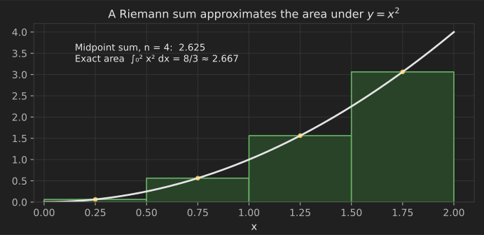
Example: For $\int_0^2 x^2\,dx$ with 4 midpoint rectangles of width 0.5: $0.5(0.0625 + 0.5625 + 1.5625 + 3.0625) = 2.625$. The exact value is $\tfrac{8}{3} \approx 2.667$.

42. Properties of the definite integral

$$\int_a^b (cf + g) = c\int_a^b f + \int_a^b g, \qquad \int_a^b f = \int_a^c f + \int_c^b f, \qquad \int_b^a f = -\int_a^b f$$

Example: Since $\sin x$ is odd, $\int_{-\pi}^{\pi}\sin x\,dx = 0$: the areas above and below the axis cancel.

43. Fundamental theorem of calculus, part 1

If $f$ is continuous, $\displaystyle\frac{d}{dx}\int_a^x f(t)\,dt = f(x)$. With a variable upper limit $g(x)$, multiply by $g'(x)$.

Example: $\displaystyle\frac{d}{dx}\int_0^{x^2}\cos(t^2)\,dt = \cos(x^4) \cdot 2x$, even though $\cos(t^2)$ has no elementary antiderivative.

44. Fundamental theorem of calculus, part 2

$$\int_a^b f(x)\,dx = F(b) - F(a) \quad\text{where } F' = f$$

Example: $\int_1^3 x^2\,dx = \frac{27}{3} - \frac{1}{3} = \frac{26}{3}$.

45. Antiderivatives to know by heart

$$\int\sec^2 x\,dx = \tan x + C, \quad \int\frac{dx}{1 + x^2} = \arctan x + C, \quad \int\frac{dx}{\sqrt{1 - x^2}} = \arcsin x + C$$

Example: $\int_0^1\frac{dx}{1 + x^2} = \arctan 1 = \frac{\pi}{4}$.

46. Substitution

$$\int f(g(x))\,g'(x)\,dx = \int f(u)\,du, \quad u = g(x)$$

Example: With $u = x^2$, $\int_0^1 xe^{x^2}\,dx = \frac{1}{2}\int_0^1 e^u\,du = \frac{e - 1}{2}$. Change the limits along with the variable.

47. Integration by parts

$$\int u\,dv = uv - \int v\,du$$

Example: $\int xe^x\,dx$ with $u = x$, $dv = e^xdx$: $xe^x - \int e^x\,dx = (x - 1)e^x + C$. Also $\int\ln x\,dx = x\ln x - x + C$ (take $u = \ln x$, $dv = dx$).

48. Repeated integration by parts

When a polynomial multiplies an exponential or trig function, apply parts until the polynomial disappears.

Example: $\int x^2e^x\,dx = e^x(x^2 - 2x + 2) + C$. Check by differentiating: $e^x(x^2 - 2x + 2) + e^x(2x - 2) = x^2e^x$.

49. Powers of sine and cosine

Use $\sin^2 x = \frac{1 - \cos 2x}{2}$ and $\cos^2 x = \frac{1 + \cos 2x}{2}$.

Example: $\int_0^{\pi}\sin^2 x\,dx = \left[\frac{x}{2} - \frac{\sin 2x}{4}\right]_0^{\pi} = \frac{\pi}{2}$.

50. Trigonometric substitution

For $\sqrt{a^2 - x^2}$ use $x = a\sin\theta$; for $\sqrt{a^2 + x^2}$, $x = a\tan\theta$; for $\sqrt{x^2 - a^2}$, $x = a\sec\theta$.

Example: With $x = \sin\theta$, $\int_0^1\sqrt{1 - x^2}\,dx = \int_0^{\pi/2}\cos^2\theta\,d\theta = \frac{\pi}{4}$: a quarter of the unit disk.

51. Partial fractions

Split a rational function into simpler fractions before integrating.

Example: $\dfrac{1}{x^2 - 1} = \dfrac{1}{2}\left(\dfrac{1}{x - 1} - \dfrac{1}{x + 1}\right)$, so $\displaystyle\int\frac{dx}{x^2 - 1} = \frac{1}{2}\ln\left|\frac{x - 1}{x + 1}\right| + C$.

52. Convergent improper integrals

$$\int_1^\infty\frac{dx}{x^p} = \frac{1}{p - 1} \quad\text{for } p > 1$$

Example: $\int_1^\infty\frac{dx}{x^2} = \lim_{b \to \infty}\left(1 - \frac{1}{b}\right) = 1$. An infinitely long region can have finite area.

53. Divergent improper integrals and the Gaussian integral

For $p \le 1$ the integral above diverges: $\int_1^\infty\frac{dx}{x} = \lim_{b \to \infty}\ln b = \infty$. A famous convergent one:

$$\int_{-\infty}^{\infty}e^{-x^2}\,dx = \sqrt{\pi}$$

Example: This is why the normal distribution's density contains $\frac{1}{\sqrt{2\pi}}$ (see formula 83 for the proof).

54. Average value of a function

$$f_{\text{avg}} = \frac{1}{b - a}\int_a^b f(x)\,dx$$

Example: The average of $\sin x$ over $[0, \pi]$ is $\frac{1}{\pi}\int_0^\pi\sin x\,dx = \frac{2}{\pi} \approx 0.637$.

55. Area between curves

$$A = \int_a^b\left[f(x) - g(x)\right]dx, \quad f \ge g$$

Example: Between $y = x$ and $y = x^2$ on $[0, 1]$: $\int_0^1(x - x^2)\,dx = \frac{1}{2} - \frac{1}{3} = \frac{1}{6}$.

56. Volume by disks

$$V = \pi\int_a^b[f(x)]^2\,dx$$

Example: Rotating $y = \sqrt{x}$, $0 \le x \le 4$, about the $x$-axis: $V = \pi\int_0^4 x\,dx = 8\pi$.

57. Volume by cylindrical shells

$$V = 2\pi\int_a^b x\,f(x)\,dx \quad\text{(rotation about the } y\text{-axis)}$$

Example: Rotating $y = x - x^2$, $0 \le x \le 1$, about the $y$-axis: $V = 2\pi\int_0^1(x^2 - x^3)\,dx = 2\pi\left(\frac{1}{3} - \frac{1}{4}\right) = \frac{\pi}{6}$.

58. Arc length

$$L = \int_a^b\sqrt{1 + [f'(x)]^2}\,dx$$

Example: For $y = \frac{2}{3}x^{3/2}$ on $[0, 3]$, $f'(x) = \sqrt{x}$, so $L = \int_0^3\sqrt{1 + x}\,dx = \frac{2}{3}\left(8 - 1\right) = \frac{14}{3}$.

59. Work done by a variable force

$$W = \int_a^b F(x)\,dx$$

Example: A spring with $k = 50$ N/m obeys $F = kx$. Stretching it 0.2 m from rest takes $W = \int_0^{0.2}50x\,dx = 25(0.04) = 1$ J.

60. Trapezoidal rule and Simpson's rule

$$T_n = \frac{h}{2}\left[f_0 + 2f_1 + \cdots + 2f_{n-1} + f_n\right], \qquad S_n = \frac{h}{3}\left[f_0 + 4f_1 + 2f_2 + \cdots + 4f_{n-1} + f_n\right]$$

Example: $\int_0^1\frac{4}{1 + x^2}\,dx = \pi$. With $n = 2$ ($h = 0.5$, values $4, 3.2, 2$): $T_2 = 3.1$ and $S_2 = \frac{1}{6}(4 + 12.8 + 2) \approx 3.1333$, against $\pi \approx 3.1416$. Simpson's rule is exact for cubics.

Sequences and series

61. Geometric series

$$\sum_{n=0}^{\infty}ar^n = \frac{a}{1 - r}, \quad |r| < 1$$

Example: $0.\overline{9} = \sum_{n=1}^\infty 9 \cdot 10^{-n} = \frac{0.9}{1 - 0.1} = 1$.

62. Divergence test and the harmonic series

If $a_n \not\to 0$, $\sum a_n$ diverges. The converse fails: $a_n \to 0$ does not guarantee convergence.

Example: The harmonic series $\sum\frac{1}{n}$ has terms going to 0 but diverges. Grouping terms, $\frac{1}{3} + \frac{1}{4} > \frac{1}{2}$, $\frac{1}{5} + \cdots + \frac{1}{8} > \frac{1}{2}$, and so on forever.

63. p-series and the Basel problem

$\sum\frac{1}{n^p}$ converges exactly when $p > 1$. Euler found the value for $p = 2$:

$$\sum_{n=1}^\infty\frac{1}{n^2} = \frac{\pi^2}{6} \approx 1.6449$$

Example: $\sum\frac{1}{n^{1.01}}$ converges, though very slowly; $\sum\frac{1}{\sqrt{n}}$ diverges.

64. Integral test

If $f$ is positive, continuous and decreasing with $a_n = f(n)$, then $\sum a_n$ and $\int_1^\infty f(x)\,dx$ both converge or both diverge.

Example: $\sum\frac{1}{n\ln n}$ (from $n = 2$) diverges because $\int_2^\infty\frac{dx}{x\ln x} = \lim_{b \to \infty}\ln(\ln b) = \infty$.

65. Comparison test

If $0 \le a_n \le b_n$ and $\sum b_n$ converges, so does $\sum a_n$.

Example: $\frac{1}{n^2 + 1} < \frac{1}{n^2}$, so $\sum\frac{1}{n^2 + 1}$ converges.

66. Ratio test

If $\lim\left|\frac{a_{n+1}}{a_n}\right| = L$: $L < 1$ converges absolutely, $L > 1$ diverges, $L = 1$ is inconclusive.

Example: For $\sum\frac{n}{2^n}$, the ratio is $\frac{n + 1}{2n} \to \frac{1}{2}$, so it converges (its sum is 2).

67. Alternating series test

If $b_n$ decreases to 0, $\sum(-1)^{n+1}b_n$ converges, and the error after $N$ terms is at most $b_{N+1}$.

Example: $1 - \frac{1}{2} + \frac{1}{3} - \cdots = \ln 2 \approx 0.6931$. After 100 terms the error is below $\frac{1}{101}$.

68. Absolute and conditional convergence

A series converges absolutely if $\sum|a_n|$ converges; it converges conditionally if it converges but not absolutely.

Example: The alternating harmonic series in formula 67 converges conditionally. By the Riemann rearrangement theorem its terms can be reordered to sum to any number you like, so the order of terms matters.

69. Radius of convergence of a power series

For $\sum c_n(x - a)^n$, the ratio test usually gives $R = \lim\left|\frac{c_n}{c_{n+1}}\right|$. Check the endpoints separately.

Example: $\sum\frac{x^n}{n}$ has $R = 1$. At $x = 1$ it is the harmonic series (diverges); at $x = -1$ it is alternating (converges). The interval is $[-1, 1)$.

70. Taylor and Maclaurin series

$$f(x) = \sum_{n=0}^\infty\frac{f^{(n)}(a)}{n!}(x - a)^n$$ $$e^x = \sum\frac{x^n}{n!}, \quad \sin x = \sum\frac{(-1)^nx^{2n+1}}{(2n + 1)!}, \quad \cos x = \sum\frac{(-1)^nx^{2n}}{(2n)!}$$

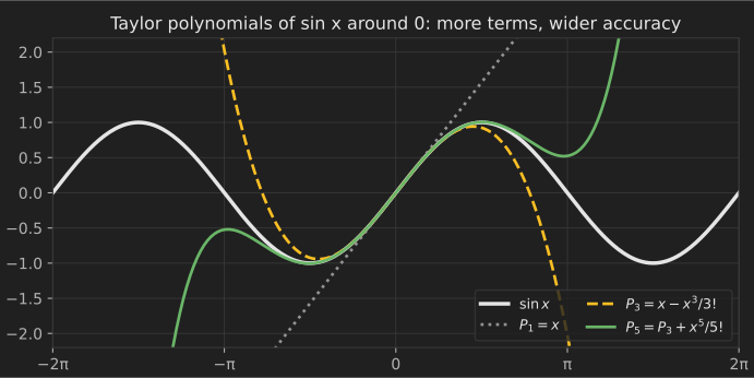
Example: $\sin 0.1 \approx 0.1 - \frac{0.001}{6} = 0.0998333$, correct to 7 decimal places.

71. Taylor's theorem with remainder

The error of the degree-$n$ Taylor polynomial is

$$R_n(x) = \frac{f^{(n+1)}(c)}{(n + 1)!}(x - a)^{n+1} \quad\text{for some } c \text{ between } a \text{ and } x$$

Example: To estimate $e$ with $\sum_{k=0}^{8}\frac{1}{k!} = 2.7182788$, the error is at most $\frac{e}{9!} < \frac{3}{362\,880} \approx 8.3 \times 10^{-6}$. The true error is about $3.0 \times 10^{-6}$.

72. Binomial series

$$(1 + x)^k = 1 + kx + \frac{k(k - 1)}{2!}x^2 + \cdots, \quad |x| < 1$$

Example: $\sqrt{1.1} = (1 + 0.1)^{1/2} \approx 1 + 0.05 - \frac{0.01}{8} = 1.04875$. The true value is $1.048809$.

Multivariable calculus

73. Partial derivatives

Differentiate with respect to one variable while holding the others fixed.

Example: For $f(x, y) = x^2y + \sin(xy)$: $f_x = 2xy + y\cos(xy)$ and $f_y = x^2 + x\cos(xy)$.

74. Gradient and directional derivative

$$\nabla f = (f_x, f_y), \qquad D_{\mathbf{u}}f = \nabla f \cdot \mathbf{u} \quad (\lVert\mathbf{u}\rVert = 1)$$

Example: $f(x, y) = x^2y$ at $(1, 2)$ has $\nabla f = (2xy, x^2) = (4, 1)$. In the direction $\mathbf{u} = (3, 4)/5$: $D_{\mathbf{u}}f = \frac{12 + 4}{5} = 3.2$.

75. The gradient points uphill

$\nabla f$ points in the direction of steepest increase, its length is the maximum rate of increase, and it is perpendicular to level curves.

Example: For $f$ in formula 74, the steepest rate at $(1, 2)$ is $\lVert(4, 1)\rVert = \sqrt{17} \approx 4.12$. Gradient descent in machine learning steps in the direction $-\nabla f$.

76. Tangent plane

$$z = f(a, b) + f_x(a, b)(x - a) + f_y(a, b)(y - b)$$

Example: For $z = x^2 + y^2$ at $(1, 2)$: $z = 5 + 2(x - 1) + 4(y - 2)$.

77. Multivariable chain rule

$$\frac{dz}{dt} = \frac{\partial z}{\partial x}\frac{dx}{dt} + \frac{\partial z}{\partial y}\frac{dy}{dt}$$

Example: $z = x^2y$ with $x = \cos t$, $y = \sin t$: $\frac{dz}{dt} = 2xy(-\sin t) + x^2\cos t = \cos t\,(1 - 3\sin^2 t)$. Backpropagation in neural networks is this rule applied through many layers.

78. Equality of mixed partials (Clairaut's theorem)

If $f_{xy}$ and $f_{yx}$ are continuous, they are equal.

Example: For $f = x^3y^2$: $f_{xy} = \frac{\partial}{\partial y}(3x^2y^2) = 6x^2y$ and $f_{yx} = \frac{\partial}{\partial x}(2x^3y) = 6x^2y$.

79. Second derivative test in two variables

At a critical point, let $D = f_{xx}f_{yy} - f_{xy}^2$. $D > 0$ and $f_{xx} > 0$: minimum. $D > 0$ and $f_{xx} < 0$: maximum. $D < 0$: saddle point.

Example: $f(x, y) = x^3 - 3x + y^2$ has critical points $(\pm 1, 0)$ and $D = 12x$. At $(1, 0)$, $D = 12 > 0$ and $f_{xx} = 6 > 0$: a local minimum. At $(-1, 0)$, $D = -12$: a saddle.

80. Lagrange multipliers

To optimize $f$ subject to $g = c$, solve $\nabla f = \lambda\nabla g$ together with $g = c$.

Example: Maximize $xy$ subject to $x + y = 10$: $(y, x) = \lambda(1, 1)$ gives $x = y = 5$ and a maximum product of 25. The optimization article works through the geometry with a diagram.

81. Double integrals over rectangles (Fubini's theorem)

For continuous $f$ on a rectangle, the double integral equals either iterated integral.

Example: $\iint_{[0,1]\times[0,2]}xy\,dA = \int_0^1 x\,dx\int_0^2 y\,dy = \frac{1}{2} \cdot 2 = 1$.

82. Double integrals over general regions

Describe the region with variable limits.

Example: Over the region between $y = x^2$ and $y = x$ for $0 \le x \le 1$: $\iint x\,dA = \int_0^1 x(x - x^2)\,dx = \frac{1}{3} - \frac{1}{4} = \frac{1}{12}$.

83. Polar coordinates

$$\iint_R f\,dA = \iint f(r\cos\theta, r\sin\theta)\,r\,dr\,d\theta$$

Example: The Gaussian integral: $\left(\int e^{-x^2}dx\right)^2 = \iint e^{-(x^2+y^2)}\,dA = \int_0^{2\pi}\int_0^\infty e^{-r^2}r\,dr\,d\theta = 2\pi \cdot \frac{1}{2} = \pi$, so $\int_{-\infty}^\infty e^{-x^2}dx = \sqrt{\pi}$.

84. Change of variables and the Jacobian

$$dx\,dy = \left|\frac{\partial(x, y)}{\partial(u, v)}\right|du\,dv$$

Example: For polar coordinates the Jacobian determinant is $\begin{vmatrix}\cos\theta & -r\sin\theta \\ \sin\theta & r\cos\theta\end{vmatrix} = r$. For spherical coordinates $dV = \rho^2\sin\phi\,d\rho\,d\phi\,d\theta$.

85. Triple integrals

Example: The volume of a ball of radius $R$ in spherical coordinates:

$$\int_0^{2\pi}\int_0^{\pi}\int_0^R\rho^2\sin\phi\,d\rho\,d\phi\,d\theta = 2\pi \cdot 2 \cdot \frac{R^3}{3} = \frac{4}{3}\pi R^3$$

86. Center of mass

$$\bar{x} = \frac{1}{A}\iint_R x\,dA, \qquad \bar{y} = \frac{1}{A}\iint_R y\,dA$$

Example: For a half-disk of radius $r$ above the $x$-axis, $\iint y\,dA = \int_0^\pi\int_0^r\rho^2\sin\theta\,d\rho\,d\theta = \frac{2r^3}{3}$ and $A = \frac{\pi r^2}{2}$, so $\bar{y} = \frac{4r}{3\pi} \approx 0.42r$.

87. Line integrals and conservative fields

If $\mathbf{F} = \nabla\phi$, then $\int_C\mathbf{F} \cdot d\mathbf{r} = \phi(\text{end}) - \phi(\text{start})$ for any path.

Example: $\mathbf{F} = (y, x) = \nabla(xy)$. The work from $(0, 0)$ to $(1, 2)$ along any path is $1 \cdot 2 - 0 = 2$.

88. Green's theorem

$$\oint_C P\,dx + Q\,dy = \iint_R\left(\frac{\partial Q}{\partial x} - \frac{\partial P}{\partial y}\right)dA$$

Example: With $P = -y/2$ and $Q = x/2$ the integrand is 1, so $\frac{1}{2}\oint(x\,dy - y\,dx)$ is the area enclosed. For a circle $x = r\cos t$, $y = r\sin t$, it gives $\frac{1}{2}\int_0^{2\pi}r^2\,dt = \pi r^2$. A planimeter measures area this way.

Vector calculus

89. Divergence and curl

$$\nabla \cdot \mathbf{F} = \frac{\partial F_1}{\partial x} + \frac{\partial F_2}{\partial y} + \frac{\partial F_3}{\partial z}, \qquad \nabla \times \mathbf{F} = \begin{vmatrix}\mathbf{i} & \mathbf{j} & \mathbf{k} \\ \partial_x & \partial_y & \partial_z \\ F_1 & F_2 & F_3\end{vmatrix}$$

Example: For $\mathbf{F} = (x^2, xy, z)$: $\nabla \cdot \mathbf{F} = 2x + x + 1 = 3x + 1$ and $\nabla \times \mathbf{F} = (0, 0, y)$. Divergence measures outflow from a point; curl measures rotation.

90. Divergence theorem

$$\iint_S\mathbf{F} \cdot \mathbf{n}\,dS = \iiint_V\nabla \cdot \mathbf{F}\,dV$$

Example: For $\mathbf{F} = (x, y, z)$ and the unit ball, $\nabla \cdot \mathbf{F} = 3$, so the flux is $3 \cdot \frac{4}{3}\pi = 4\pi$. Directly: on the unit sphere $\mathbf{F} \cdot \mathbf{n} = 1$, and the area is $4\pi$. Gauss's law for electric fields is this theorem.

91. Stokes' theorem

$$\oint_C\mathbf{F} \cdot d\mathbf{r} = \iint_S(\nabla \times \mathbf{F}) \cdot \mathbf{n}\,dS$$

Example: $\mathbf{F} = (-y, x, 0)$ has curl $(0, 0, 2)$. Over the unit disk, $\iint 2\,dA = 2\pi$, which equals the circulation $\oint(-y\,dx + x\,dy) = \int_0^{2\pi}1\,dt = 2\pi$ around the unit circle.

92. Test for a conservative field

On a simply connected region, a smooth field is conservative exactly when its curl is zero (in 2D: $\partial Q/\partial x = \partial P/\partial y$).

Example: $\mathbf{F} = (2xy, x^2)$: $\partial_x(x^2) = 2x = \partial_y(2xy)$, so $\mathbf{F} = \nabla(x^2y)$. Gravity and electrostatic fields are conservative, which is why potential energy is well defined.

Differential equations

93. Exponential growth and decay

$$\frac{dy}{dt} = ky \quad\Longrightarrow\quad y = y_0e^{kt}$$

Example: Carbon-14 has a half-life of about 5,730 years, so $k = -\frac{\ln 2}{5730}$. A sample with 25% of its original carbon-14 is two half-lives old, about 11,460 years.

94. Newton's law of cooling

$$\frac{dT}{dt} = -k(T - T_{\text{room}}) \quad\Longrightarrow\quad T = T_{\text{room}} + (T_0 - T_{\text{room}})e^{-kt}$$

Example: Coffee at 90 °C in a 20 °C room cools to 60 °C in 10 minutes, so $e^{-10k} = \frac{40}{70}$ and $k \approx 0.0560$ per minute. It reaches 40 °C when $e^{-kt} = \frac{20}{70}$, at $t = \frac{\ln 3.5}{k} \approx 22.4$ minutes.

95. Logistic growth

$$\frac{dP}{dt} = rP\left(1 - \frac{P}{K}\right) \quad\Longrightarrow\quad P(t) = \frac{K}{1 + \frac{K - P_0}{P_0}e^{-rt}}$$

Example: Growth is fastest when $P = K/2$, where the curve has its inflection point. Populations, technology adoption and the spread of rumors often follow this S-shaped curve.

96. First-order linear equations (integrating factor)

For $y' + p(x)y = q(x)$, multiply by $\mu = e^{\int p\,dx}$; then $(\mu y)' = \mu q$.

Example: $y' + y = x$: $\mu = e^x$, $(e^xy)' = xe^x$, so $e^xy = (x - 1)e^x + C$ and $y = x - 1 + Ce^{-x}$.

97. Second-order linear equations with constant coefficients

For $ay'' + by' + cy = 0$, try $y = e^{rx}$ and solve $ar^2 + br + c = 0$.

Example: $y'' - 3y' + 2y = 0$ gives $r = 1, 2$, so $y = c_1e^x + c_2e^{2x}$.

98. Simple harmonic motion

$$my'' + ky = 0 \quad\Longrightarrow\quad y = A\cos(\omega t) + B\sin(\omega t), \quad \omega = \sqrt{k/m}$$

Example: A 0.5 kg mass on a spring with $k = 8$ N/m oscillates with $\omega = 4$ rad/s and period $\frac{2\pi}{4} = \frac{\pi}{2} \approx 1.57$ s.

99. Damped oscillations

$my'' + by' + ky = 0$ has characteristic roots $r = \frac{-b \pm \sqrt{b^2 - 4mk}}{2m}$. Underdamped ($b^2 < 4mk$) systems oscillate while decaying; critically damped ($b^2 = 4mk$) systems return fastest without oscillating.

Example: For the spring in formula 98, critical damping needs $b = \sqrt{4 \cdot 0.5 \cdot 8} = 4$ N·s/m. Car shock absorbers are designed to be close to critically damped.

100. Euler's method

$$y_{n+1} = y_n + h\,f(x_n, y_n)$$

Example: For $y' = y$, $y(0) = 1$ and step $h = 0.25$, four steps give $y(1) \approx 1.25^4 = 2.441$, against the exact $e \approx 2.718$. Halving $h$ roughly halves the error, which is why practical solvers use higher-order methods such as Runge–Kutta.

Common mistakes

• Using a theorem without its hypotheses. The mean value theorem needs continuity on the closed interval and differentiability inside; L'Hôpital's rule only applies to $0/0$ or $\infty/\infty$ forms.
• Dropping the inner derivative in the chain rule. $\frac{d}{dx}\sin(x^2) = 2x\cos(x^2)$, not $\cos(x^2)$.
• Forgetting to change the limits in a substitution. Either change them to $u$-values or substitute back before evaluating.
• Assuming $a_n \to 0$ means the series converges. The harmonic series is the standard counterexample (formula 62).
• Forgetting the Jacobian. In polar coordinates $dA = r\,dr\,d\theta$, not $dr\,d\theta$.
• Treating an improper integral as ordinary. $\int_{-1}^1\frac{dx}{x^2}$ is not $-2$; the integrand blows up at 0 and the integral diverges.
• Using degrees. Every derivative and series of a trigonometric function in this article assumes radians.

Next steps

• See derivatives, gradients and Lagrange multipliers put to work in 100 mathematical optimization techniques used in AI, engineering and research.
• Use integrals as probabilities in 101 probability and statistics concepts for data science and machine learning.
• Review prerequisites in 100 mathematics formulas every student should know, or practise matrices in 101 linear algebra problems with solutions.
• Explore how calculus feeds into Fourier analysis and dynamical systems in 100 advanced mathematics concepts with real-world applications, and browse the mathematics category.

References

• Calculus Volume 1, Gilbert Strang and Edwin "Jed" Herman, OpenStax (2016). https://openstax.org/books/calculus-volume-1/pages/4-4-the-mean-value-theorem
• Calculus Volume 2, Gilbert Strang and Edwin "Jed" Herman, OpenStax (2016). https://openstax.org/books/calculus-volume-2/pages/6-3-taylor-and-maclaurin-series
• Calculus Volume 3, Gilbert Strang and Edwin "Jed" Herman, OpenStax (2016). https://openstax.org/books/calculus-volume-3/pages/6-8-the-divergence-theorem
• Active Calculus, Matthew Boelkins, open textbook. https://activecalculus.org/
• NIST Digital Library of Mathematical Functions, National Institute of Standards and Technology, §4.28 (hyperbolic functions). https://dlmf.nist.gov/4.28
• Elementary Differential Equations and Boundary Value Problems, William E. Boyce, Richard C. DiPrima and Douglas B. Meade, Wiley, 12th edition (2021).