100 Best Mathematical Optimization Techniques Used in AI, Engineering, and Research

Optimization is the mathematics of choosing the best option under constraints. Training a neural network, routing delivery vans, designing a lighter bracket, allocating an investment portfolio, scheduling power plants and tuning hyperparameters are all optimization problems. They differ in whether variables are continuous or discrete, whether the objective is smooth or noisy, whether constraints exist, and, most of all, whether the problem is convex.

This guide collects 100 techniques grouped by the kind of problem they solve: the foundations, classical methods for smooth unconstrained problems, constrained optimization, linear and convex programming, combinatorial optimization, global and derivative-free methods, the optimizers that train modern AI models, and applications in engineering and research. For each technique you get the core idea, the key formula where there is one, when to use it, and a small example. Numerical examples were recomputed with Python (NumPy and SciPy).

Prerequisites are gradients, Hessians and Lagrange multipliers from multivariable calculus; 100 calculus formulas, theorems and examples covers them.

Foundations

1. The standard form of an optimization problem

$$\min_{\mathbf{x} \in \mathbb{R}^n} f(\mathbf{x}) \quad\text{subject to}\quad g_i(\mathbf{x}) \le 0,\; h_j(\mathbf{x}) = 0$$

$f$ is the objective, $\mathbf{x}$ the decision variables, $g_i$ and $h_j$ the inequality and equality constraints. Maximizing $f$ is minimizing $-f$.

Example: Choose production quantities $\mathbf{x}$ to minimize cost, subject to meeting demand ($h_j$) and machine capacity ($g_i$).

2. Local and global minima

$\mathbf{x}^*$ is a global minimum if $f(\mathbf{x}^*) \le f(\mathbf{x})$ for every feasible $\mathbf{x}$, and a local minimum if this holds only nearby. Most practical algorithms only guarantee local minima.

3. Convex sets

A set is convex if the line segment between any two of its points stays inside it. Intersections of convex sets are convex, which is why problems whose constraints are linear inequalities have convex feasible regions.

4. Convex functions

$f$ is convex if $f(\theta\mathbf{x} + (1 - \theta)\mathbf{y}) \le \theta f(\mathbf{x}) + (1 - \theta)f(\mathbf{y})$: every chord lies above the graph. For a convex function, every local minimum is global, which is why convexity is the dividing line between "easy" and "hard" optimization.

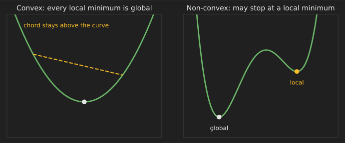
Example: $x^2$, $e^x$, $|x|$, norms, and the logistic regression loss are convex; $\sin x$ and most neural network losses are not.

5. First-order optimality condition

At an unconstrained local minimum of a differentiable function, $\nabla f(\mathbf{x}^*) = \mathbf{0}$. For convex $f$ this condition is also sufficient.

Example: $f(x) = (x - 3)^2$ has $f'(x) = 2(x - 3) = 0$ at $x = 3$.

6. Second-order conditions and the Hessian

If $\nabla f(\mathbf{x}^*) = \mathbf{0}$ and the Hessian $\nabla^2 f(\mathbf{x}^*)$ is positive definite, $\mathbf{x}^*$ is a strict local minimum. An indefinite Hessian means a saddle point.

Example: $f(x, y) = x^2 - y^2$ has a zero gradient at the origin, but its Hessian $\operatorname{diag}(2, -2)$ is indefinite: a saddle.

7. Lipschitz smoothness

$f$ is $L$-smooth if its gradient changes at most at rate $L$: $\lVert\nabla f(\mathbf{x}) - \nabla f(\mathbf{y})\rVert \le L\lVert\mathbf{x} - \mathbf{y}\rVert$. For a quadratic, $L$ is the largest Hessian eigenvalue. It sets the largest safe step size for gradient descent.

8. Strong convexity

$f$ is $\mu$-strongly convex if it curves upward at least as fast as $\frac{\mu}{2}\lVert\mathbf{x}\rVert^2$. Strong convexity guarantees a unique minimizer and lets gradient descent converge at a geometric (linear) rate.

9. Condition number

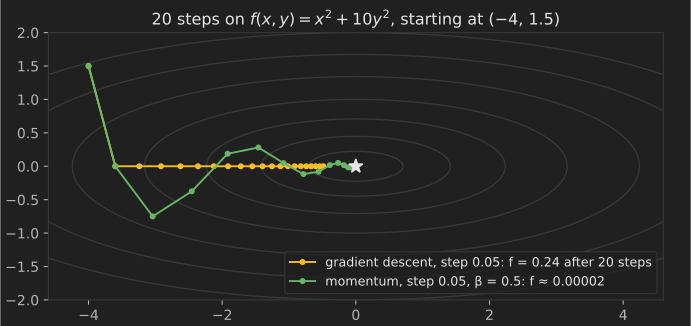
$\kappa = L / \mu$, the ratio of the steepest to the shallowest curvature. Large $\kappa$ means long, narrow valleys where gradient methods zigzag.

Example: $f(x, y) = x^2 + 10y^2$ has Hessian $\operatorname{diag}(2, 20)$, so $\kappa = 10$. Rescaling $y$ to make the valley round (preconditioning) would make $\kappa = 1$.

10. Problem classes and their difficulty

Linear programs, convex quadratic programs and general convex problems can be solved to global optimality efficiently. General non-convex and integer problems are NP-hard in the worst case, so practice relies on structure, good starting points and heuristics. Identifying the class is the most important step in choosing a method.

Classical methods for smooth problems

11. Golden-section search

For a unimodal function of one variable, shrink a bracketing interval by the factor $0.618$ (the inverse golden ratio) each step, reusing one interior point.

Example: After 20 iterations an interval of length 1 shrinks to $0.618^{20} \approx 6.6 \times 10^{-5}$, with no derivatives required.

12. Gradient descent

$$\mathbf{x}_{k+1} = \mathbf{x}_k - \eta\,\nabla f(\mathbf{x}_k)$$

Step downhill, with step size (learning rate) $\eta$.

Example: For $f(x) = (x - 3)^2$ with $\eta = 0.1$ from $x_0 = 0$, each step multiplies the distance to 3 by $0.8$, so $x_k = 3(1 - 0.8^k)$ and $x_{10} \approx 2.68$.

13. Choosing the step size

For an $L$-smooth function, any fixed step $\eta < 2/L$ makes gradient descent on a convex quadratic converge, and $\eta = 1/L$ is the standard safe choice. Too large and iterates diverge; too small and progress crawls.

Example: For $x^2 + 10y^2$, $L = 20$, so $\eta$ must be below 0.1. At $\eta = 0.11$ the $y$-coordinate is multiplied by $1 - 0.11 \times 20 = -1.2$ each step and blows up.

14. Backtracking line search (Armijo rule)

Start with a large step and shrink it by a factor (say 0.5) until $f(\mathbf{x} - \eta\nabla f) \le f(\mathbf{x}) - c\,\eta\lVert\nabla f\rVert^2$ with a small $c$ such as $10^{-4}$. It adapts the step automatically and is standard in classical solvers.

15. Newton's method

$$\mathbf{x}_{k+1} = \mathbf{x}_k - \left[\nabla^2 f(\mathbf{x}_k)\right]^{-1}\nabla f(\mathbf{x}_k)$$

It fits a quadratic model and jumps to its minimum. Near a well-behaved minimum it converges quadratically: the number of correct digits roughly doubles each step.

Example: Minimizing $f(x) = x - \ln x$ (minimum at $x = 1$) gives the update $x_{k+1} = 2x_k - x_k^2$. From $x_0 = 0.5$: $0.75$, $0.9375$, $0.99609$, $0.9999847$.

16. Gauss–Newton method

For nonlinear least squares $\min\sum r_i(\mathbf{x})^2$, approximate the Hessian by $J^{T}J$, where $J$ is the Jacobian of the residuals. Each step solves a linear least-squares problem, with no second derivatives needed.

17. Levenberg–Marquardt algorithm

Blend Gauss–Newton and gradient descent: solve $(J^{T}J + \lambda I)\boldsymbol{\delta} = -J^{T}\mathbf{r}$, increasing $\lambda$ when a step fails and decreasing it when it succeeds.

Example: SciPy's curve_fit uses Levenberg–Marquardt by default for unbounded problems. It is the workhorse for fitting models to experimental data and for camera calibration.

18. BFGS quasi-Newton method

Build an approximation of the inverse Hessian from successive gradient differences, so you get near-Newton convergence (superlinear) using only gradients.

19. L-BFGS

Limited-memory BFGS stores only the last few (typically 5 to 20) gradient-difference pairs instead of an $n \times n$ matrix, so it scales to millions of variables.

Example: The default solver for logistic regression in scikit-learn is L-BFGS (solver="lbfgs").

20. Conjugate gradient method

For a symmetric positive definite system $A\mathbf{x} = \mathbf{b}$ (equivalently minimizing $\tfrac{1}{2}\mathbf{x}^{T}A\mathbf{x} - \mathbf{b}^{T}\mathbf{x}$), choose search directions that are mutually $A$-conjugate. In exact arithmetic it finishes in at most $n$ steps, and it needs only matrix-vector products.

Example: Large sparse systems from finite-element simulations are solved with preconditioned conjugate gradients.

21. Coordinate descent

Minimize over one variable (or block) at a time, holding the others fixed. Very effective when each one-dimensional problem has a closed form.

Example: Lasso and elastic-net regression in scikit-learn and glmnet are solved by coordinate descent with soft-thresholding (technique 31).

22. Nelder–Mead simplex method

A derivative-free method that moves a simplex of $n + 1$ points by reflecting, expanding and contracting it. Useful for small, noisy problems where gradients are unavailable; it has no general convergence guarantee and scales poorly beyond a few dozen variables. (It is unrelated to the simplex method for linear programming.)

23. Trust-region methods

Instead of choosing a direction then a step length, minimize a quadratic model within a region $\lVert\boldsymbol{\delta}\rVert \le \Delta$ where the model is trusted, then grow or shrink $\Delta$ depending on how well the model predicted the actual decrease. Robust when the Hessian is indefinite.

Constrained optimization

24. Lagrange multipliers

To optimize $f$ subject to $h(\mathbf{x}) = 0$, solve $\nabla f = \lambda\nabla h$ with $h = 0$. At the optimum the level curve of $f$ is tangent to the constraint.

Example: Minimize $x^2 + y^2$ subject to $x + y = 2$: $(2x, 2y) = \lambda(1, 1)$ gives $x = y = 1$, $\lambda = 2$ and minimum value 2.

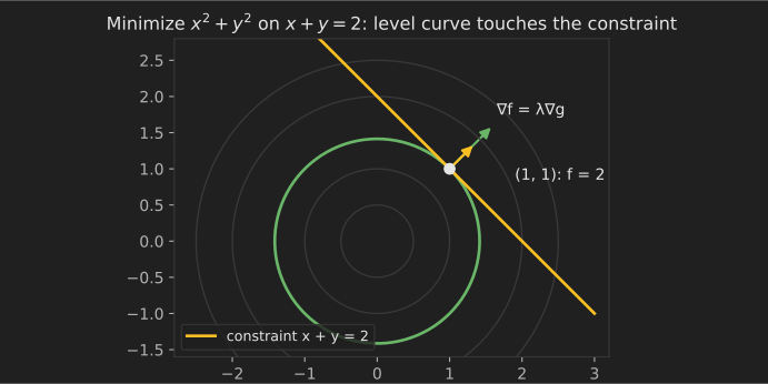
The multiplier has a meaning: it is the rate at which the optimal value changes as the constraint is relaxed. Raising the constant 2 to $c$ gives optimal value $c^2/2$, whose derivative at $c = 2$ is $2 = \lambda$.

25. Karush–Kuhn–Tucker (KKT) conditions

For inequality constraints $g_i \le 0$, the optimum (under mild regularity conditions) satisfies: stationarity $\nabla f + \sum\mu_i\nabla g_i + \sum\lambda_j\nabla h_j = \mathbf{0}$, primal feasibility, dual feasibility $\mu_i \ge 0$, and complementary slackness $\mu_ig_i = 0$.

Example: Minimize $(x - 2)^2$ subject to $x \le 1$. The constraint is active at $x = 1$, and stationarity $2(1 - 2) + \mu = 0$ gives $\mu = 2 \ge 0$. Complementary slackness says a constraint that is not tight has a zero multiplier.

26. Lagrangian duality

The dual function $d(\boldsymbol{\lambda}, \boldsymbol{\mu}) = \min_{\mathbf{x}}L(\mathbf{x}, \boldsymbol{\lambda}, \boldsymbol{\mu})$ gives a lower bound on the optimal value (weak duality). For convex problems satisfying Slater's condition, the bound is tight (strong duality). Dual problems are sometimes easier, and support vector machines are usually trained through theirs.

27. Penalty methods

Replace constraints with a penalty: minimize $f(\mathbf{x}) + \rho\sum h_j(\mathbf{x})^2$ and increase $\rho$. Simple, but large $\rho$ makes the problem badly conditioned.

28. Augmented Lagrangian method

Combine a Lagrange multiplier term with a quadratic penalty, then update the multiplier after each minimization: $\boldsymbol{\lambda} \leftarrow \boldsymbol{\lambda} + \rho\,h(\mathbf{x})$. It converges without driving $\rho$ to infinity.

29. ADMM

The alternating direction method of multipliers splits $\min f(\mathbf{x}) + g(\mathbf{z})$ subject to $A\mathbf{x} + B\mathbf{z} = \mathbf{c}$ into alternating updates of $\mathbf{x}$, $\mathbf{z}$ and the multiplier. Each subproblem is often simple and can be distributed across machines (Boyd et al., 2011).

30. Projected gradient descent

Take a gradient step, then project back onto the feasible set: $\mathbf{x}_{k+1} = \Pi_C(\mathbf{x}_k - \eta\nabla f(\mathbf{x}_k))$. Efficient whenever projection is cheap.

Example: Projecting onto box constraints $0 \le x_i \le 1$ just clips each coordinate.

31. Proximal gradient method and soft-thresholding

For $f(\mathbf{x}) + \lambda\lVert\mathbf{x}\rVert_1$ with smooth $f$, take a gradient step on $f$, then apply the proximal operator of the $\ell_1$ norm, soft-thresholding:

$$S_\lambda(x) = \operatorname{sign}(x)\max(|x| - \lambda, 0)$$

Example: With $\lambda = 1$, $S_1(3) = 2$ and $S_1(0.5) = 0$. Small coefficients become exactly zero, which is how the lasso selects features (the ISTA algorithm; FISTA adds momentum).

32. Interior-point (barrier) methods

Replace $g_i(\mathbf{x}) \le 0$ with a barrier term $-\frac{1}{t}\sum\log(-g_i(\mathbf{x}))$ that blows up at the boundary, then follow the solutions as $t \to \infty$ (the central path) using Newton steps. Interior-point methods solve linear, quadratic and semidefinite programs in polynomial time and are the default in many commercial solvers.

33. Sequential quadratic programming (SQP)

At each step, solve a quadratic program built from a quadratic model of the Lagrangian and linearized constraints. Among the most effective methods for smooth nonlinear constrained problems, such as trajectory optimization.

Example: SciPy's minimize(method="SLSQP") is an SQP implementation.

34. Frank–Wolfe (conditional gradient) method

Instead of projecting, minimize the linear approximation of $f$ over the feasible set and move toward that point. It keeps iterates sparse and avoids projections, which helps when the feasible set is, for example, the probability simplex or a set of low-rank matrices.

35. Active-set methods

Guess which inequality constraints are tight, solve the resulting equality-constrained problem, and update the guess. Efficient for small and medium quadratic programs, and well suited to warm starts in repeated solves such as model predictive control (technique 90).

Linear and convex programming

36. Linear programming

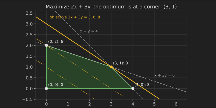
Minimize or maximize a linear objective subject to linear constraints. If an optimum exists, one occurs at a vertex of the feasible polygon (or polytope).

Example: Maximize $2x + 3y$ subject to $x + y \le 4$, $x + 3y \le 6$, $x, y \ge 0$. The vertices give $0$, $8$, $9$ and $6$, so the optimum is $9$ at $(3, 1)$.

37. The simplex method

Dantzig's method (1947) walks from vertex to adjacent vertex, improving the objective each step. Its worst case is exponential (Klee and Minty, 1972), but in practice it is fast and remains central to commercial solvers, especially for re-solving after small changes.

38. LP duality and shadow prices

Every LP has a dual LP whose optimal value equals the primal's. The dual variables are shadow prices: the value of one more unit of each resource.

Example: The dual of technique 36 is: minimize $4u + 6v$ subject to $u + v \ge 2$, $u + 3v \ge 3$, $u, v \ge 0$. Its solution is $u = 1.5$, $v = 0.5$ with value $4(1.5) + 6(0.5) = 9$, matching the primal. One more unit of the first resource is worth 1.5.

39. Integer programming and branch and bound

When variables must be integers, solve the LP relaxation, pick a fractional variable, and branch into two subproblems ($x \le \lfloor x^* \rfloor$ and $x \ge \lceil x^* \rceil$). Prune any branch whose relaxation bound is worse than the best integer solution found so far.

40. Mixed-integer programming (MIP)

Some variables continuous, some integer: yes/no decisions (open a warehouse, start a generator) combined with continuous quantities. Modern solvers combine branch and bound with cutting planes, presolve and heuristics, and solve industrial instances with millions of variables.

41. Cutting planes

Add linear inequalities that every integer solution satisfies but the current fractional LP solution violates, tightening the relaxation. Gomory cuts (1958) are the classic family.

42. Quadratic programming and portfolio optimization

Minimize a convex quadratic subject to linear constraints. Markowitz (1952) portfolio selection minimizes variance $\mathbf{w}^{T}\Sigma\mathbf{w}$ for a target return.

Example: Two uncorrelated assets with volatilities 20% and 30%: the minimum-variance weight on the first is $\frac{0.3^2}{0.2^2 + 0.3^2} \approx 0.692$, giving portfolio volatility about 16.6%, lower than either asset alone.

43. Least squares as optimization

$\min\lVert A\mathbf{x} - \mathbf{b}\rVert^2$ has the closed-form solution of the normal equations, but is best solved by QR or SVD for numerical stability. Ridge regression adds $\lambda\lVert\mathbf{x}\rVert^2$, giving $(A^{T}A + \lambda I)\mathbf{x} = A^{T}\mathbf{b}$.

Example: Worked fits appear in 101 linear algebra problems with solutions (problems 95 and 96).

44. Second-order cone programming (SOCP)

Constraints of the form $\lVert A\mathbf{x} + \mathbf{b}\rVert_2 \le \mathbf{c}^{T}\mathbf{x} + d$. Covers robust linear programs, antenna array design and some grasping problems in robotics, and is solved efficiently by interior-point methods.

45. Semidefinite programming (SDP)

Optimize a linear objective over positive semidefinite matrices. Used for control design (linear matrix inequalities), and the Goemans–Williamson algorithm uses it to approximate max-cut within a factor of about 0.878.

46. Geometric programming

Problems with posynomial objectives and constraints become convex after a logarithmic change of variables. Used in digital circuit sizing and aircraft conceptual design.

47. Disciplined convex programming tools

Modeling languages such as CVXPY (Python) and JuMP (Julia) let you state a convex problem close to its mathematical form, verify convexity by construction, and pass it to an appropriate solver.

Combinatorial and discrete optimization

48. Dynamic programming

Break a problem into overlapping subproblems with optimal substructure and store each subproblem's answer. Bellman's principle of optimality: every tail of an optimal plan is optimal for its own subproblem.

Example: The 0/1 knapsack problem with capacity $W$ fills a table $V[i][w]$ in $O(nW)$ time. Edit distance, sequence alignment and the Viterbi algorithm are all dynamic programs.

49. Greedy algorithms

Make the locally best choice at each step. Optimal for some problems (minimum spanning trees, Huffman coding, the fractional knapsack) and only heuristic for others.

Example: Knapsack capacity 50 with items (weight, value) $(10, 60)$, $(20, 100)$, $(30, 120)$. Greedy by value per kilogram takes the first two for 160; the optimum takes the last two for 220.

50. Shortest paths

Dijkstra's algorithm finds shortest paths from a source in graphs with non-negative edge weights; Bellman–Ford handles negative weights; A* adds a heuristic to search toward a goal. Every navigation app runs a variant. A worked example appears in 100 advanced mathematics concepts with real-world applications.

51. Minimum spanning trees

Connect all nodes with minimum total edge weight using Kruskal's or Prim's greedy algorithm. Used in network design and as a building block in clustering and approximation algorithms.

52. Maximum flow and minimum cut

The maximum flow from source to sink equals the capacity of the smallest cut separating them (the max-flow min-cut theorem). Algorithms such as Edmonds–Karp and push–relabel solve it. Applications include bipartite matching, image segmentation and network reliability.

53. The assignment problem

Assign $n$ workers to $n$ tasks at minimum total cost. The Hungarian algorithm solves it in $O(n^3)$.

Example: For costs $\begin{bmatrix} 4 & 1 & 3 \\ 2 & 0 & 5 \\ 3 & 2 & 2 \end{bmatrix}$, the optimum assigns worker 1 to task 2, worker 2 to task 1 and worker 3 to task 3, for a total of $1 + 2 + 2 = 5$ (SciPy's linear_sum_assignment).

54. Traveling salesman heuristics

The number of distinct tours of $n$ cities is $(n - 1)!/2$: 181,440 for 10 cities and about $6 \times 10^{16}$ for 20. Exact solvers (Concorde) use cutting planes and branch and bound; practical routing uses construction heuristics plus local improvements such as 2-opt, which reverses a segment of the tour whenever that shortens it.

55. Constraint programming

Declare variables, domains and constraints, then search with propagation that prunes impossible values. Strong for scheduling and timetabling, where constraints are complex and logical rather than linear.

56. Local search

Start from a solution and repeatedly move to a better neighbor. Fast and general, but it stops at local optima, which motivates the metaheuristics below.

Global and derivative-free optimization

57. Simulated annealing

Accept a worse move with probability $e^{-\Delta/T}$, where $\Delta$ is the increase in cost and the temperature $T$ decreases over time (Kirkpatrick, Gelatt and Vecchi, 1983).

Example: A move that worsens cost by 2 is accepted with probability $e^{-2} \approx 0.14$ at $T = 1$, but $e^{-0.2} \approx 0.82$ at $T = 10$. Early on the search explores; later it settles.

58. Genetic algorithms

Evolve a population of candidate solutions with selection, crossover and mutation. Flexible for messy discrete or mixed problems, though usually less sample-efficient than methods that exploit problem structure.

59. Particle swarm optimization

Particles move through the search space, pulled toward their own best position and the swarm's best position (Kennedy and Eberhart, 1995). Simple to implement for continuous black-box problems.

60. CMA-ES

The covariance matrix adaptation evolution strategy samples candidates from a multivariate normal distribution and adapts its mean and covariance toward successful steps. One of the strongest general-purpose methods for difficult continuous black-box problems with up to a few hundred variables.

61. Tabu search

A local search that forbids recently visited moves for a while (the tabu list), forcing the search out of local optima. Widely used in vehicle routing and scheduling.

62. Multistart

Run a local optimizer from many random starting points and keep the best result. Crude but effective, and easy to parallelize.

63. Bayesian optimization

For expensive black-box functions, fit a probabilistic surrogate (often a Gaussian process) to the evaluations so far, and choose the next point by maximizing an acquisition function such as expected improvement, which balances exploring uncertain regions and exploiting promising ones.

Example: Tuning a model's hyperparameters when each training run takes hours, or choosing the next experiment in materials or drug discovery.

64. Random search versus grid search

When only a few hyperparameters really matter, random search covers each important dimension more thoroughly than a grid with the same budget (Bergstra and Bengio, 2012).

Example: With 60 random trials, the chance that at least one lands in the best 5% of the search space is $1 - 0.95^{60} \approx 95\%$, regardless of the number of dimensions.

Optimization for machine learning and AI

65. Empirical risk minimization

Training a model means minimizing the average loss over the training data:

$$\min_{\boldsymbol{\theta}}\frac{1}{n}\sum_{i=1}^n\ell\big(f_{\boldsymbol{\theta}}(\mathbf{x}_i), y_i\big) + \lambda R(\boldsymbol{\theta})$$

The real goal is low error on unseen data, so the optimizer that minimizes training loss fastest is not always the one that generalizes best.

66. Loss functions

Mean squared error for regression, cross-entropy for classification, hinge loss $\max(0, 1 - y\,f(\mathbf{x}))$ for support vector machines, Huber loss for regression with outliers. The choice of loss defines what "best" means; see the probability interpretation in 101 probability and statistics concepts for data science.

67. Stochastic gradient descent (SGD)

Replace the full gradient with the gradient on one example or a small batch. Each step is noisy but cheap, and the noise can help escape poor regions. With decreasing step sizes it converges for convex problems.

68. Mini-batch training

Average gradients over a batch of $B$ examples. Larger batches give less noisy gradients and better hardware utilization, with diminishing returns: gradient noise falls like $1/\sqrt{B}$.

69. Momentum

$$\mathbf{v}_{k+1} = \beta\mathbf{v}_k + \nabla f(\mathbf{x}_k), \qquad \mathbf{x}_{k+1} = \mathbf{x}_k - \eta\,\mathbf{v}_{k+1}$$

Accumulate a running direction so consistent gradients add up and oscillating components cancel. With $\beta = 0.9$, a steady gradient is effectively amplified by $1/(1 - \beta) = 10$.

70. Nesterov accelerated gradient

Evaluate the gradient at the look-ahead point $\mathbf{x}_k - \eta\beta\mathbf{v}_k$ instead of $\mathbf{x}_k$. For smooth convex problems it achieves the optimal rate for first-order methods, $O(1/k^2)$ versus $O(1/k)$ for gradient descent (Nesterov, 1983).

71. AdaGrad

Scale each parameter's step by the inverse square root of its accumulated squared gradients, so rarely updated parameters get larger steps (Duchi, Hazan and Singer, 2011). Good for sparse features, but the step size shrinks forever.

72. RMSProp

Like AdaGrad, but with an exponential moving average of squared gradients so the effective step size does not decay to zero. Proposed by Geoffrey Hinton in his 2012 Coursera lecture notes.

73. Adam

Combine momentum (first moment $\mathbf{m}$) with RMSProp scaling (second moment $\mathbf{v}$), with bias correction for the zero initialization (Kingma and Ba, 2014):

$$\mathbf{m}_t = \beta_1\mathbf{m}_{t-1} + (1 - \beta_1)\mathbf{g}_t, \quad \mathbf{v}_t = \beta_2\mathbf{v}_{t-1} + (1 - \beta_2)\mathbf{g}_t^2, \quad \boldsymbol{\theta}_t = \boldsymbol{\theta}_{t-1} - \eta\frac{\hat{\mathbf{m}}_t}{\sqrt{\hat{\mathbf{v}}_t} + \epsilon}$$

where $\hat{\mathbf{m}}_t = \mathbf{m}_t / (1 - \beta_1^t)$ and $\hat{\mathbf{v}}_t = \mathbf{v}_t / (1 - \beta_2^t)$. Common defaults are $\eta = 10^{-3}$, $\beta_1 = 0.9$, $\beta_2 = 0.999$ and $\epsilon = 10^{-8}$.

74. AdamW (decoupled weight decay)

In Adam, adding an L2 penalty to the loss gets distorted by the adaptive scaling. AdamW applies weight decay directly to the parameters, $\boldsymbol{\theta} \leftarrow \boldsymbol{\theta} - \eta\lambda\boldsymbol{\theta}$, separately from the gradient step (Loshchilov and Hutter, 2019). It is the usual default for training transformers.

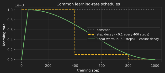
75. Learning-rate schedules

Large steps early make fast progress; small steps late settle into a minimum. Common schedules are step decay, exponential decay, cosine decay and one-cycle.

76. Learning-rate warmup

Start with a tiny learning rate and increase it linearly over the first few hundred or thousand steps. It stabilizes training while Adam's moment estimates and the network's activations settle, and is standard for transformers and large-batch training.

77. Gradient clipping

If the gradient norm exceeds a threshold $c$, rescale it: $\mathbf{g} \leftarrow c\,\mathbf{g}/\lVert\mathbf{g}\rVert$.

Example: With $c = 1$, the gradient $(3, 4)$ (norm 5) becomes $(0.6, 0.8)$. Clipping prevents single bad batches from destroying training, especially in recurrent networks and large language models.

78. Early stopping

Track validation loss and stop (or keep the best checkpoint) when it stops improving. It acts as a regularizer: for linear models trained with gradient descent it behaves much like an L2 penalty.

79. Backpropagation and automatic differentiation

Reverse-mode automatic differentiation computes the gradient of a scalar loss with respect to millions of parameters at a cost of a small constant multiple of one forward pass, by applying the chain rule backward through the computation graph. It is what makes gradient-based training of deep networks practical.

80. Weight initialization

Initialize weights so that activations and gradients keep roughly constant variance through layers: Xavier/Glorot initialization uses variance $\frac{2}{n_{\text{in}} + n_{\text{out}}}$ for tanh-like activations (Glorot and Bengio, 2010); He initialization uses $\frac{2}{n_{\text{in}}}$ for ReLU (He et al., 2015). Poor initialization causes vanishing or exploding gradients.

81. Saddle points in high dimensions

In high-dimensional non-convex losses, most critical points with high loss are saddle points rather than poor local minima, because it is unlikely that every direction curves upward (Dauphin et al., 2014). Gradient noise and momentum help escape them.

82. Sharp versus flat minima

Very large batches tend to converge to sharper minima that may generalize worse (Keskar et al., 2016). The link between flatness and generalization is still debated, because sharpness depends on how the parameters are scaled. Methods such as sharpness-aware minimization (SAM) explicitly seek flatter regions.

83. Large-batch training and the linear scaling rule

When multiplying the batch size by $k$, multiply the learning rate by $k$ and use warmup. Goyal et al. (2017) trained ResNet-50 on ImageNet with batch size 8,192 in one hour this way without losing accuracy.

84. Mixed-precision training and loss scaling

Compute in 16-bit floating point for speed and memory while keeping a 32-bit master copy of the weights. Multiply the loss by a scale factor before backpropagation so small gradients do not underflow, then unscale before the update (Micikevicius et al., 2018).

85. Successive halving and Hyperband

Start many hyperparameter configurations on a small budget, keep the best fraction, give them more budget, and repeat. Hyperband (Li et al., 2018) runs several such brackets to hedge against how early performance predicts final performance.

86. Policy gradient methods

In reinforcement learning, optimize expected reward $J(\boldsymbol{\theta}) = E[R]$ using $\nabla J = E\left[R\,\nabla\log\pi_{\boldsymbol{\theta}}(a \mid s)\right]$ (REINFORCE; Williams, 1992). Practical versions subtract a baseline to reduce variance and limit the size of each policy update, as in proximal policy optimization (PPO).

87. Preconditioned and second-order optimizers for deep learning

Methods such as K-FAC (Martens and Grosse, 2015) and Shampoo (Gupta et al., 2018) approximate curvature with structured matrices per layer, taking better-scaled steps than diagonal methods like Adam at extra cost per step. They are an active research area for large-scale training.

88. Support vector machines as optimization

The soft-margin SVM solves

$$\min_{\mathbf{w}, b}\frac{1}{2}\lVert\mathbf{w}\rVert^2 + C\sum_i\max\left(0, 1 - y_i(\mathbf{w}^{T}\mathbf{x}_i + b)\right)$$

a convex quadratic program. Its dual depends on the data only through dot products, which allows kernels.

Optimization in engineering and research

89. Linear–quadratic regulator (LQR)

For linear dynamics $\dot{\mathbf{x}} = A\mathbf{x} + B\mathbf{u}$ and cost $\int(\mathbf{x}^{T}Q\mathbf{x} + \mathbf{u}^{T}R\mathbf{u})\,dt$, the optimal control is linear feedback $\mathbf{u} = -K\mathbf{x}$, with $K$ computed from the algebraic Riccati equation. Used to balance inverted pendulums, stabilize aircraft and tune many industrial controllers.

90. Model predictive control (MPC)

At every time step, solve an optimization over a finite future horizon subject to constraints, apply only the first control action, then re-solve with new measurements. It handles constraints such as actuator limits and is used in chemical plants, autonomous driving and building climate control.

91. Bellman equation and optimal control

$$V(s) = \max_a\left[r(s, a) + \gamma\sum_{s'}P(s' \mid s, a)V(s')\right]$$

The value of a state is the best immediate reward plus the discounted value of where you land. Value iteration and policy iteration solve it; reinforcement learning approximates it from experience.

92. Topology optimization

Decide where material should exist inside a design region to make a structure as stiff as possible for a given mass. The SIMP method treats each element's density as a continuous variable penalized toward 0 or 1, and solves with gradients from finite-element analysis. It produces the organic-looking brackets seen in aerospace and additive manufacturing.

93. Multi-objective optimization and Pareto fronts

When objectives conflict (cost versus weight, accuracy versus latency), a solution is Pareto optimal if no objective can improve without another getting worse. Methods include weighted sums, the $\varepsilon$-constraint method and evolutionary algorithms such as NSGA-II, which return a whole front for the decision-maker to choose from.

94. Robust optimization

Optimize the worst case over an uncertainty set for uncertain parameters, so the solution stays feasible when data deviate from nominal values. For many uncertainty sets the robust version of a linear program is still a tractable convex problem (often an SOCP).

95. Stochastic programming

Optimize expected cost over scenarios, often in two stages: decide now (build capacity), then adapt after uncertainty is revealed (dispatch). Used in energy planning, supply chains and finance.

96. Inverse problems and Tikhonov regularization

Recovering causes from effects (deblurring an image, reconstructing a CT scan, locating an earthquake) is often ill-posed: small noise causes large errors. Tikhonov regularization solves $\min\lVert A\mathbf{x} - \mathbf{b}\rVert^2 + \lambda\lVert L\mathbf{x}\rVert^2$, trading a small bias for stability. Ridge regression is the special case $L = I$.

97. Compressed sensing and L1 minimization

If a signal is sparse in some basis, it can often be recovered from far fewer measurements than its length by minimizing $\lVert\mathbf{x}\rVert_1$ subject to matching the measurements (Candès, Romberg and Tao, 2006; Donoho, 2006). This has shortened MRI scan times.

98. Optimal transport and the Sinkhorn algorithm

Find the cheapest way to move one probability distribution onto another. Adding an entropy term turns the linear program into a problem solved by alternately rescaling rows and columns of a matrix (Cuturi, 2013). Used in domain adaptation, comparing distributions and generative modeling.

99. Bilevel optimization

An outer problem whose constraints include the solution of an inner optimization problem. Hyperparameter tuning (inner: train weights; outer: minimize validation loss), meta-learning and leader–follower pricing games are bilevel. Gradients of the outer problem can be obtained by differentiating through the inner solution or its optimality conditions.

100. The adjoint method for design optimization

To get the gradient of one objective with respect to thousands of design parameters in a simulation governed by differential equations, solve one extra adjoint equation instead of one simulation per parameter. It is the engineering counterpart of backpropagation and drives aerodynamic shape optimization of wings and turbine blades.

Choosing a technique

Common mistakes

• Using a local method on a non-convex problem and trusting the answer as global. Try several starting points, or prove convexity.
• Picking the learning rate by habit. Run a short learning-rate sweep; too large diverges and too small wastes compute (technique 13).
• Ignoring scaling. Features or variables on wildly different scales create ill-conditioned problems (technique 9). Standardize or precondition.
• Rounding an LP solution to get an integer solution. The result can be infeasible or far from optimal; use a MIP solver.
• Reporting the best of many tuning runs as expected performance. Hyperparameter search overfits the validation set; confirm on a separate test set.
• Forgetting constraints that exist in reality. An optimizer will exploit any missing constraint, such as negative production or physically impossible designs.

Next steps

• Review gradients, Hessians and Lagrange multipliers in 100 calculus formulas, theorems and examples.
• Practise the linear algebra behind least squares, conditioning and SVD in 101 linear algebra problems with solutions and 101 linear algebra concepts for machine learning.
• Connect losses to likelihoods in 101 probability and statistics concepts for data science and machine learning.
• Try scikit-learn's optimizers in Python machine learning examples, and browse the mathematics and engineering categories.

References

• Convex Optimization, Stephen Boyd and Lieven Vandenberghe, Cambridge University Press (2004). Free PDF: https://web.stanford.edu/~boyd/cvxbook/
• Numerical Optimization, Jorge Nocedal and Stephen J. Wright, Springer, 2nd edition (2006).
• Deep Learning, Ian Goodfellow, Yoshua Bengio and Aaron Courville, MIT Press (2016), chapter 8, "Optimization for Training Deep Models". https://www.deeplearningbook.org/contents/optimization.html
• Boyd, S., Parikh, N., Chu, E., Peleato, B. and Eckstein, J. (2011). "Distributed Optimization and Statistical Learning via the Alternating Direction Method of Multipliers." Foundations and Trends in Machine Learning, 3(1). https://web.stanford.edu/~boyd/papers/admm_distr_stats.html
• Kingma, D. P. and Ba, J. (2014). "Adam: A Method for Stochastic Optimization." arXiv:1412.6980. https://arxiv.org/abs/1412.6980
• Loshchilov, I. and Hutter, F. (2019). "Decoupled Weight Decay Regularization." ICLR. arXiv:1711.05101. https://arxiv.org/abs/1711.05101
• Duchi, J., Hazan, E. and Singer, Y. (2011). "Adaptive Subgradient Methods for Online Learning and Stochastic Optimization." JMLR, 12. https://www.jmlr.org/papers/v12/duchi11a.html
• Goyal, P. et al. (2017). "Accurate, Large Minibatch SGD: Training ImageNet in 1 Hour." arXiv:1706.02677. https://arxiv.org/abs/1706.02677
• Bergstra, J. and Bengio, Y. (2012). "Random Search for Hyper-Parameter Optimization." JMLR, 13. https://www.jmlr.org/papers/v13/bergstra12a.html
• Li, L., Jamieson, K., DeSalvo, G., Rostamizadeh, A. and Talwalkar, A. (2018). "Hyperband: A Novel Bandit-Based Approach to Hyperparameter Optimization." JMLR, 18. https://jmlr.org/papers/v18/16-558.html
• Keskar, N. S. et al. (2016). "On Large-Batch Training for Deep Learning: Generalization Gap and Sharp Minima." arXiv:1609.04836. https://arxiv.org/abs/1609.04836
• Micikevicius, P. et al. (2018). "Mixed Precision Training." ICLR. arXiv:1710.03740. https://arxiv.org/abs/1710.03740
• Dauphin, Y. et al. (2014). "Identifying and attacking the saddle point problem in high-dimensional non-convex optimization." arXiv:1406.2572. https://arxiv.org/abs/1406.2572
• Cuturi, M. (2013). "Sinkhorn Distances: Lightspeed Computation of Optimal Transport." arXiv:1306.0895. https://arxiv.org/abs/1306.0895
• Kirkpatrick, S., Gelatt, C. D. and Vecchi, M. P. (1983). "Optimization by Simulated Annealing." Science, 220(4598), 671–680. https://doi.org/10.1126/science.220.4598.671
• CVXPY documentation. https://www.cvxpy.org/