100 Best Advanced Mathematics Concepts Explained With Real-World Applications

Much of the mathematics taught after calculus can look like abstraction for its own sake: groups, manifolds, measure theory, Hilbert spaces. Yet the phone in your pocket encrypts messages with number theory, compresses photos with Fourier and wavelet analysis, fixes scratched data with finite fields, locates itself with relativity's geometry, and runs apps compiled by tools built on logic and graph theory.

This article explains 100 advanced concepts across twelve areas of mathematics. Each entry says what the idea is, in plain language and with the key formula where one helps, and then where it is used in the real world. Small worked examples were checked with Python (SymPy, NumPy and SciPy). The goal is orientation, not a full course: each entry is a pointer to a subject you can study in depth.

Number theory and cryptography

1. Modular arithmetic

Arithmetic where numbers wrap around after reaching a modulus: $a \equiv b \pmod{n}$ when $n$ divides $a - b$.

Applications: clock and calendar calculations, hash tables, checksums such as ISBN and IBAN check digits, and every public-key cryptosystem.

Example: $17 \equiv 5 \pmod{12}$: 17:00 is 5 o'clock.

2. The Euclidean algorithm

$\gcd(a, b) = \gcd(b, a \bmod b)$, repeated until the remainder is 0. It is one of the oldest algorithms still in daily use, and it runs in a number of steps proportional to the number of digits.

Example: $\gcd(252, 105)$: $252 = 2 \cdot 105 + 42$, $105 = 2 \cdot 42 + 21$, $42 = 2 \cdot 21$, so the gcd is 21.

3. Bézout's identity and modular inverses

There are integers $x, y$ with $ax + by = \gcd(a, b)$. When $\gcd(a, n) = 1$, this gives the inverse of $a$ modulo $n$.

Applications: computing RSA private keys (concept 8) and solving linear congruences.

Example: $3 \cdot 4 = 12 \equiv 1 \pmod{11}$, so $3^{-1} \equiv 4 \pmod{11}$.

4. Fermat's little theorem

If $p$ is prime and $p \nmid a$, then $a^{p-1} \equiv 1 \pmod{p}$.

Applications: fast probabilistic primality tests (Fermat and Miller–Rabin) used when generating cryptographic keys.

5. Euler's totient theorem

$a^{\varphi(n)} \equiv 1 \pmod{n}$ when $\gcd(a, n) = 1$, where $\varphi(n)$ counts integers up to $n$ coprime to $n$. For $n = pq$ with distinct primes, $\varphi(n) = (p - 1)(q - 1)$. This is the theorem that makes RSA decryption work.

6. Chinese remainder theorem

A system of congruences with pairwise coprime moduli has exactly one solution modulo their product.

Example: $x \equiv 2 \pmod 3$, $x \equiv 3 \pmod 5$, $x \equiv 2 \pmod 7$ has the unique solution $x \equiv 23 \pmod{105}$.

Applications: speeding up RSA decryption by about four times, and computer arithmetic that splits large numbers into residues processed in parallel.

7. The prime number theorem

The number of primes up to $x$ is approximately $\pi(x) \approx \frac{x}{\ln x}$.

Example: There are 78,498 primes below one million, against the estimate $\frac{10^6}{\ln 10^6} \approx 72{,}382$; the logarithmic integral $\operatorname{li}(x)$ is much closer. The theorem tells key generators how long to search: random 1024-bit numbers are prime with probability about $1/710$.

8. RSA public-key encryption

Choose primes $p, q$, set $n = pq$, pick $e$ coprime to $\varphi(n)$ and compute $d = e^{-1} \bmod \varphi(n)$. Encrypt with $c = m^e \bmod n$, decrypt with $m = c^d \bmod n$. Security rests on the difficulty of factoring $n$.

Example (toy numbers): $p = 61$, $q = 53$, $n = 3233$, $\varphi(n) = 3120$, $e = 17$, $d = 2753$. The message $m = 65$ encrypts to $65^{17} \bmod 3233 = 2790$, and $2790^{2753} \bmod 3233 = 65$. Real keys use primes hundreds of digits long.

9. Discrete logarithms and Diffie–Hellman key exchange

Given $g$ and $g^a \bmod p$, finding $a$ is believed to be hard. Two parties exchange $g^a$ and $g^b$ publicly and both compute the shared secret $g^{ab}$.

Example (toy numbers): $p = 23$, $g = 5$, secrets $a = 6$ and $b = 15$. The public values are $5^6 \bmod 23 = 8$ and $5^{15} \bmod 23 = 19$, and both sides compute $19^6 \equiv 8^{15} \equiv 2 \pmod{23}$.

10. Elliptic curve cryptography

Points on a curve $y^2 = x^3 + ax + b$ over a finite field form a group, and the discrete logarithm problem in that group is much harder than in ordinary modular arithmetic. A 256-bit elliptic-curve key gives security comparable to a 3,072-bit RSA key (NIST SP 800-57).

Applications: HTTPS key exchange, Signal and other secure messengers, and cryptocurrency signatures.

Abstract algebra

11. Groups

A set with an associative operation, an identity and inverses. Groups are the mathematics of symmetry: the symmetries of any object form a group.

Example: The rotations of a square by 0°, 90°, 180° and 270° form a group of order 4.

12. Symmetry groups in chemistry and crystallography

Every crystal belongs to one of 230 space groups, and every repeating wallpaper pattern to one of 17 wallpaper groups. Molecular symmetry groups predict which vibrations show up in infrared and Raman spectra.

13. The Rubik's cube group

The cube's legal positions form a group with $43{,}252{,}003{,}274{,}489{,}856{,}000$ elements. In 2010 a computer search showed that every position can be solved in at most 20 moves ("God's number").

14. Finite fields

Number systems with finitely many elements where you can add, subtract, multiply and divide (except by zero). For every prime power $p^k$ there is exactly one, written $\mathrm{GF}(p^k)$.

Applications: AES encryption does its byte arithmetic in $\mathrm{GF}(2^8)$; elliptic curve cryptography and error-correcting codes also live in finite fields.

15. Hamming codes

Add parity bits in positions that are powers of 2, so the pattern of failed parity checks spells out the position of a single flipped bit. The Hamming(7,4) code sends 4 data bits in 7 and corrects any single-bit error.

Applications: error-correcting (ECC) memory in servers.

16. Reed–Solomon codes

Treat data as coefficients of a polynomial over a finite field and send extra evaluations of it; any $k$ correct values determine the polynomial. They correct bursts of errors.

Applications: CDs, DVDs and Blu-ray discs, QR codes (which stay readable when partly damaged), deep-space probes and RAID 6 storage.

17. Rings, ideals and polynomial algebra

Rings generalize the integers; ideals generalize multiples. Gröbner bases turn systems of polynomial equations into a form that can be solved step by step.

Applications: computer algebra systems, robot inverse kinematics and geometric theorem proving.

18. Galois theory

It links the symmetries of the roots of a polynomial to whether the polynomial can be solved by radicals. It proves there is no general formula like the quadratic formula for polynomials of degree 5 or higher (the Abel–Ruffini theorem), and that some classical constructions, such as trisecting an arbitrary angle with straightedge and compass, are impossible.

Advanced linear algebra

19. Eigenvectors and PageRank

Google's original PageRank scores pages by the stationary distribution of a random surfer, which is the dominant eigenvector of a modified link matrix (with damping factor 0.85 in the original paper).

Applications: web search, citation ranking and influence scores in social networks.

20. Singular value decomposition

Every matrix factors as $A = U\Sigma V^{T}$: rotate, stretch, rotate. Truncating to the largest singular values gives the best low-rank approximation.

Applications: recommender systems (latent factors from the Netflix Prize era), image compression and noise reduction. Worked examples: 101 linear algebra problems with solutions, problems 99 and 100.

21. Principal component analysis

Find the orthogonal directions of greatest variance in data (eigenvectors of the covariance matrix) and keep the top few.

Applications: visualizing high-dimensional data, face recognition (eigenfaces) and summarizing genetic variation across populations.

22. Markov chains

A system that moves between states with probabilities depending only on the current state. Long-run behavior is the eigenvector with eigenvalue 1 of the transition matrix.

Applications: queue models, credit-rating migration, text generation, and Markov chain Monte Carlo sampling in statistics.

23. Tensor decompositions

Generalizations of SVD to arrays with three or more indices (CP and Tucker decompositions).

Applications: analyzing user × item × time data, chemometrics (fluorescence spectroscopy), and compressing neural network layers.

24. Spectral graph theory

The eigenvalues and eigenvectors of a graph's Laplacian matrix $L = D - A$ reveal its structure: the number of zero eigenvalues equals the number of connected components, and the second eigenvector suggests a good way to cut the graph in two.

Applications: spectral clustering, image segmentation and graph neural networks.

Analysis and Fourier methods

25. Metric spaces and completeness

A metric space has a notion of distance; it is complete if every Cauchy sequence converges. Completeness is what guarantees that iterative algorithms which "settle down" actually converge to something in the space.

26. Banach fixed-point theorem

On a complete metric space, a contraction (a map that shrinks distances by a factor $q < 1$) has exactly one fixed point, and iterating it from anywhere converges there.

Applications: proving that PageRank's power iteration converges, that value iteration in reinforcement learning works, and that solutions to many differential equations exist and are unique (Picard–Lindelöf).

27. Measure theory and the Lebesgue integral

A rigorous way to assign "size" to sets and integrate very irregular functions. It is the foundation of modern probability: a probability is a measure with total mass 1.

Applications: the rigorous basis for expected values, stochastic calculus (concept 62) and convergence theorems used in statistics and machine learning theory.

28. Fourier series

A periodic function can be written as a sum of sines and cosines:

$$f(x) = \frac{a_0}{2} + \sum_{n=1}^{\infty}\left(a_n\cos nx + b_n\sin nx\right)$$

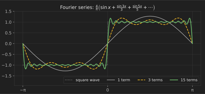
Applications: analyzing musical tones and vibrations, and solving the heat equation (Fourier's original motivation, 1822).

29. The Fourier transform

$$\hat{f}(\xi) = \int_{-\infty}^{\infty} f(t)\,e^{-2\pi i \xi t}\,dt$$

It converts a signal from time to frequency. Convolution in time becomes multiplication in frequency.

Applications: audio equalizers, MRI image reconstruction, spectroscopy and radio.

30. The fast Fourier transform

The Cooley–Tukey algorithm (1965) computes the discrete Fourier transform of $N$ points in $O(N\log N)$ operations instead of $O(N^2)$.

Example: For $N = 2^{20}$ (about a million) samples, that is roughly 52,000 times fewer operations. FFTs run inside Wi-Fi and 4G/5G modems (OFDM), and in fast multiplication of huge integers.

31. The discrete cosine transform

A Fourier-type transform using only cosines, whose coefficients concentrate the energy of smooth image blocks into a few numbers.

Applications: JPEG images and MP3/AAC audio compress by keeping the large coefficients and discarding the rest.

32. Laplace transform

$$F(s) = \int_0^\infty f(t)\,e^{-st}\,dt$$

It turns linear differential equations into algebraic equations.

Applications: analyzing electrical circuits, and the transfer functions that control engineers use to design autopilots, cruise control and thermostats.

33. Wavelets

Basis functions that are localized in both time and frequency, so they capture short events and sharp edges better than sines.

Applications: JPEG 2000 image compression, the FBI's fingerprint compression standard, denoising signals and detecting transients in ECGs.

34. Hilbert spaces

Complete vector spaces with an inner product, possibly infinite-dimensional, where geometry (lengths, angles, projections) still works.

Applications: quantum mechanics describes physical states as vectors in a Hilbert space; signal processing and kernel methods in machine learning rely on the same geometry.

Complex analysis

35. Complex numbers as rotations

Multiplying by $i$ rotates a point in the complex plane by $90^\circ$; multiplying by $re^{i\theta}$ scales by $r$ and rotates by $\theta$.

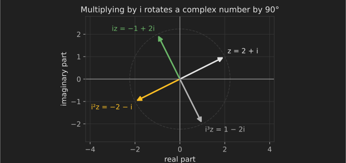
Applications: 2D graphics and signal processing use complex multiplication as a compact way to rotate and phase-shift.

36. Euler's formula

$$e^{i\theta} = \cos\theta + i\sin\theta, \qquad e^{i\pi} + 1 = 0$$

It ties exponentials to oscillation, which is why waves, AC circuits and quantum amplitudes are written as complex exponentials.

37. Phasors in AC circuits

Represent a sinusoidal voltage $V_0\cos(\omega t + \phi)$ by the complex number $V_0e^{i\phi}$. Capacitors and inductors become complex impedances $\frac{1}{i\omega C}$ and $i\omega L$, and circuit analysis reduces to Ohm's law with complex numbers.

Applications: power grid analysis, filter design and audio electronics.

38. Conformal maps

Analytic functions preserve angles locally. The Joukowski map $w = z + \frac{1}{z}$ turns circles into airfoil shapes, so flow around a cylinder (easy) becomes flow around a wing (hard).

Applications: early aerodynamics, electrostatics and map projections (the Mercator projection is conformal).

39. The residue theorem

The integral of an analytic function around a closed curve equals $2\pi i$ times the sum of residues at the singularities inside.

Applications: evaluating difficult real integrals, inverting Laplace and z-transforms, and stability analysis of control systems (the Nyquist criterion).

40. Fractals and the Mandelbrot set

The Mandelbrot set is the set of complex $c$ for which iterating $z_{n+1} = z_n^2 + c$ from $z_0 = 0$ stays bounded. Its boundary has infinitely intricate detail.

Applications: fractal geometry models natural shapes (coastlines, ferns, blood vessels), and fractal antenna designs fit multiple frequency bands into a small device.

Differential equations and dynamical systems

41. Ordinary differential equations as models

An ODE relates a quantity to its rate of change. Most dynamic models in science and engineering, from drug concentrations in the body to orbits and circuits, are ODEs. The core techniques are in 100 calculus formulas, theorems and examples.

42. The SIR epidemic model

$$\frac{dS}{dt} = -\beta SI, \qquad \frac{dI}{dt} = \beta SI - \gamma I, \qquad \frac{dR}{dt} = \gamma I$$

The basic reproduction number $R_0 = \beta / \gamma$ decides whether an outbreak grows ($R_0 > 1$). In this simplest model, the herd-immunity threshold is $1 - 1/R_0$.

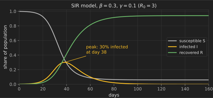
Applications: public-health planning. Real models add age structure, contact networks, waning immunity and interventions.

43. Predator–prey (Lotka–Volterra) equations

$$\frac{dx}{dt} = \alpha x - \beta xy, \qquad \frac{dy}{dt} = \delta xy - \gamma y$$

Prey ($x$) and predator ($y$) populations cycle, with predator peaks lagging prey peaks.

Applications: ecology, fisheries management and models of economic cycles.

44. The heat (diffusion) equation

$$\frac{\partial u}{\partial t} = \alpha\nabla^2 u$$

Heat, chemicals and probability spread from high to low concentration, smoothing out differences.

Applications: cooling electronics, drug diffusion, image denoising and the diffusion models used to generate images.

45. The wave equation

$$\frac{\partial^2 u}{\partial t^2} = c^2\nabla^2 u$$

Applications: acoustics, vibrating strings and bridges, seismic imaging for oil exploration and earthquake studies, and electromagnetic waves.

46. The Navier–Stokes equations

They describe fluid flow from conservation of mass and momentum. Whether smooth solutions always exist in three dimensions is one of the Clay Mathematics Institute's Millennium Prize Problems, with a $1 million prize.

Applications: weather forecasting, aircraft and car design, blood flow and ocean currents, through computational fluid dynamics.

47. The Schrödinger equation

$$i\hbar\frac{\partial\psi}{\partial t} = \hat{H}\psi$$

It governs how quantum states evolve.

Applications: semiconductor and laser design, chemistry simulations of molecules and materials, and quantum computing.

48. The Black–Scholes equation

A partial differential equation for the price of an option, derived by assuming the stock follows geometric Brownian motion and that the option can be hedged continuously. Scholes and Merton received the 1997 Nobel prize in economics for this work (Black had died in 1995).

Applications: options pricing and risk management, with known limits: real returns have heavier tails than the model assumes.

49. Chaos and the logistic map

The simple rule $x_{n+1} = rx_n(1 - x_n)$ settles down for some $r$, cycles for others, and becomes chaotic, never repeating and extremely sensitive to the starting value, for most $r$ beyond about 3.57.

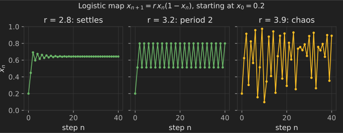
Applications: population biology, and a teaching model for why long-range prediction fails in some deterministic systems.

50. Strange attractors and the butterfly effect

Edward Lorenz's 1963 weather model ($\sigma = 10$, $\rho = 28$, $\beta = 8/3$) showed that deterministic equations can make tiny differences in initial conditions grow exponentially.

Applications: this is why weather forecasts lose skill after roughly one to two weeks, and why forecasters run ensembles of slightly perturbed simulations.

51. Bifurcation theory

Studies how a system's behavior changes qualitatively as a parameter crosses a threshold, as at $r = 3$ in the logistic map, where a steady state splits into a 2-cycle.

Applications: tipping points in climate and ecosystems, the onset of flutter in aircraft wings, and buckling in structures.

52. Stability and Lyapunov functions

An equilibrium is stable if nearby trajectories stay nearby. A Lyapunov function, an "energy" that always decreases along trajectories, proves stability without solving the equations.

Applications: certifying that controllers for drones, robots and power grids will not run away.

Numerical analysis

53. Floating-point arithmetic

Computers store real numbers with finite precision (IEEE 754). Double precision has machine epsilon $2^{-52} \approx 2.2 \times 10^{-16}$, so 0.1 + 0.2 == 0.3 is false in most languages.

Applications: understanding rounding error is essential in finance, scientific computing and any comparison of computed numbers. Compare with a tolerance, not with ==.

54. Finite differences

Approximate derivatives by differences on a grid, for example $f''(x) \approx \frac{f(x + h) - 2f(x) + f(x - h)}{h^2}$.

Applications: simulating heat flow, option prices and seismic waves on grids.

55. The finite element method

Split a complex shape into small elements (triangles, tetrahedra), approximate the solution simply on each, and assemble a large sparse linear system.

Applications: structural analysis of bridges and aircraft, crash simulation, heat transfer and biomechanics.

56. Runge–Kutta methods

Estimate the slope several times within each step and combine the estimates. The classic fourth-order method (RK4) has error proportional to $h^4$, compared with $h$ for Euler's method.

Applications: orbit calculations, circuit simulation and the default solvers in scientific libraries (SciPy's solve_ivp uses an adaptive Runge–Kutta pair by default).

57. Monte Carlo methods

Estimate quantities by random sampling; the error shrinks like $1/\sqrt{N}$ regardless of dimension.

Applications: radiation transport (Monte Carlo methods were developed at Los Alamos in the 1940s), financial risk, rendering realistic light in films (path tracing) and Bayesian statistics.

58. Conditioning and numerical stability

A problem is ill-conditioned if small input changes cause large output changes; an algorithm is unstable if it amplifies rounding error. Both must be controlled for trustworthy results.

Applications: choosing QR over the normal equations for regression, pivoting in Gaussian elimination, and reformulating formulas to avoid subtracting nearly equal numbers.

Probability and stochastic processes

59. Bayesian inference

Update beliefs with evidence: posterior ∝ likelihood × prior.

Applications: spam filters, medical diagnosis, search-and-rescue planning (the U.S. Coast Guard's SAROPS search software) and A/B testing. More in 101 probability and statistics concepts for data science.

60. Stochastic processes

Collections of random variables indexed by time, such as random walks and Poisson processes.

Applications: modeling call arrivals, insurance claims, radioactive decay and neuron firing.

61. Brownian motion

A continuous random walk with independent, normally distributed increments. Einstein's 1905 analysis of it helped confirm that atoms exist.

Applications: diffusion of particles, models of stock prices, and the noise process in diffusion-based image generators.

62. Itô calculus

Calculus for functions of Brownian motion, where $(dW)^2 = dt$ adds an extra term to the chain rule (Itô's lemma).

Applications: derivatives pricing, filtering, and stochastic differential equations in physics and biology.

63. Queueing theory

Models waiting lines. Little's law, $L = \lambda W$, says the average number in a system equals the arrival rate times the average time spent.

Example: For a single server with arrivals $\lambda = 8$ per hour and service rate $\mu = 10$ per hour (M/M/1), the average time in the system is $\frac{1}{\mu - \lambda} = 0.5$ hours and the average number present is $\lambda W = 4$. At 80% utilization, small increases in load cause large increases in waiting.

Applications: call centers, hospital emergency departments, network routers and cloud autoscaling.

64. Information theory and channel capacity

Shannon's theorem gives the maximum error-free data rate of a noisy channel:

$$C = B\log_2\left(1 + \frac{S}{N}\right)$$

Example: A 1 MHz channel with signal-to-noise ratio 1000 (30 dB) can carry at most about 9.97 Mbit/s.

Applications: the design target for every modem, Wi-Fi standard and mobile network; data compression limits come from Shannon's entropy.

65. The Kalman filter

The optimal estimator for a linear system with Gaussian noise: predict the next state, then correct the prediction with a measurement, weighted by their uncertainties.

Applications: Apollo spacecraft navigation, GPS receivers, aircraft autopilots, robot localization and smartphone sensor fusion.

66. Extreme value theory

The maxima of large samples follow one of three limiting distribution families (Gumbel, Fréchet, Weibull), combined in the generalized extreme value distribution.

Applications: setting flood-defense heights, designing structures for 100-year winds, and estimating tail risk in insurance and finance.

Discrete mathematics and graph theory

67. Graphs

Vertices connected by edges, possibly with weights and directions. Graphs model road networks, social networks, the internet, molecules, dependencies between software packages and knowledge graphs.

68. Shortest paths

Dijkstra's algorithm finds the cheapest route from a starting vertex when all edge weights are non-negative, by repeatedly settling the closest unsettled vertex.

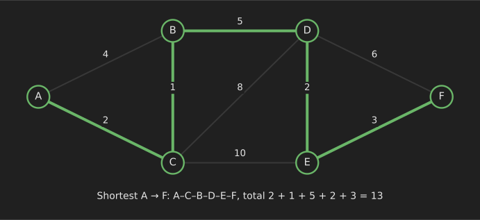
Applications: GPS navigation, internet routing protocols (OSPF) and route planning in games.

69. Network flows

Maximize flow through a network with capacity limits; the maximum flow equals the minimum cut. More in 100 mathematical optimization techniques.

Applications: logistics, airline scheduling, bipartite matching (assigning doctors to residencies) and image segmentation.

70. Graph coloring

Assign colors to vertices so that neighbors differ. The four color theorem (Appel and Haken, 1976, the first major theorem proved with essential computer help) says any planar map needs at most four.

Applications: exam timetabling (exams sharing students cannot share a slot), assigning radio frequencies, and register allocation in compilers.

71. Eulerian and Hamiltonian paths

An Eulerian path uses every edge once and exists under a simple degree condition (Euler's solution to the Königsberg bridges problem, 1736). A Hamiltonian path visits every vertex once, and deciding whether one exists is NP-complete.

Applications: route planning for snowplows and mail delivery (Eulerian), and genome assembly from DNA fragments using de Bruijn graphs.

72. Random graphs and small-world networks

Watts and Strogatz (1998) showed that adding a few random shortcuts to a regular network makes typical path lengths short while keeping local clustering high: the "six degrees of separation" effect.

Applications: epidemic spread on contact networks, the robustness of the internet, and the structure of neural and social networks.

73. The pigeonhole principle

If more than $n$ items go into $n$ boxes, some box has at least two.

Applications: proving that every lossless compression scheme must make some files larger, and that hash collisions are unavoidable.

74. Generating functions

Encode a sequence as coefficients of a power series, $\sum a_nx^n$, so that counting problems become algebra.

Applications: counting combinatorial structures, analyzing algorithm running times, and probability (moment-generating functions).

75. Recurrence relations and algorithm analysis

Divide-and-conquer algorithms satisfy recurrences such as $T(n) = 2T(n/2) + n$, whose solution $O(n\log n)$ follows from the master theorem.

Applications: predicting how merge sort, FFT and binary search scale before writing code.

76. Boolean algebra

Algebra with values 0 and 1 and operations AND, OR and NOT. Claude Shannon's 1937 master's thesis showed it describes switching circuits.

Applications: every digital circuit and processor; circuit minimization; database queries and search filters.

Logic and the theory of computation

77. Turing machines and computability

A Turing machine is a minimal model of computation. Turing (1936) proved the halting problem undecidable: no program can decide, for every program and input, whether it eventually stops.

Applications: explains why perfect bug detectors and perfect antivirus programs are impossible; real tools must accept false alarms or misses.

78. P versus NP

P is the class of problems solvable in polynomial time; NP is the class whose solutions can be checked in polynomial time. Whether P = NP is the most famous open problem in computer science and another Millennium Prize Problem.

Applications: much of cryptography assumes certain problems are hard; a proof that P = NP with a practical algorithm would upend it.

79. NP-completeness and reductions

A problem is NP-complete if it is in NP and every NP problem reduces to it. SAT, the traveling salesman decision problem, graph coloring and scheduling are examples.

Applications: recognizing NP-completeness tells engineers to use heuristics, approximations or special structure rather than search for a perfect fast algorithm. Modern SAT solvers nevertheless handle industrial instances with millions of variables in chip verification.

80. Lambda calculus

Church's 1930s model of computation using only function definition and application.

Applications: the foundation of functional programming languages (Haskell, OCaml, Lisp) and of anonymous functions (lambdas) in Python, JavaScript and Java.

81. Formal verification and proof assistants

Proof assistants such as Lean, Coq (now Rocq) and Isabelle check every step of a proof by computer.

Applications: the CompCert verified C compiler, the seL4 verified operating-system kernel, hardware verification at chip makers, and verified formal proofs of major mathematical theorems.

82. Finite automata and regular expressions

Finite automata recognize exactly the languages described by regular expressions.

Applications: text search, input validation, lexical analysis in compilers and network packet inspection.

Geometry and topology

83. Non-Euclidean geometry

Geometries in which Euclid's parallel postulate fails: on a sphere, triangle angles sum to more than 180°.

Applications: navigation on the Earth's surface, and the curved spacetime of general relativity.

84. Relativity and GPS

General relativity makes GPS satellite clocks run fast by about 45 microseconds per day relative to the ground, and special relativity makes them run slow by about 7, a net gain of about 38 microseconds per day. Uncorrected, positions would drift by roughly 10 km per day.

85. Differential geometry and curvature

Studies curves, surfaces and higher-dimensional spaces using calculus. Gaussian curvature can be measured from inside a surface (Gauss's Theorema Egregium), which is why a flat map of the Earth must distort distances or areas.

Applications: map projections, computer graphics, general relativity and the design of curved architectural shells.

86. Geodesics

The shortest paths on a curved surface. On a sphere they are great circles.

Applications: long-haul flights between Europe and North America curve toward the Arctic because that great-circle route is shorter than it looks on a flat map.

87. Topology

The study of properties preserved by continuous deformation, such as connectedness and the number of holes. For any convex polyhedron, $V - E + F = 2$ (Euler's formula).

Applications: robot motion planning, sensor-network coverage, and the topological phases of matter recognized by the 2016 Nobel Prize in Physics.

88. Knot theory

Classifies closed loops in three dimensions up to deformation, using invariants such as knot polynomials.

Applications: enzymes called topoisomerases change the knotting and linking of DNA, and knot theory helps quantify their action; it also appears in polymer physics and in proposals for topological quantum computing.

89. Topological data analysis

Persistent homology tracks which loops and voids appear and disappear as you connect nearby data points at increasing scales, summarizing the "shape" of data in a way that is robust to noise.

Applications: analyzing protein structures, materials, brain networks and sensor data.

90. Manifolds

Spaces that look locally like ordinary flat space but may be curved or twisted globally, like the surface of the Earth.

Applications: the configuration space of a robot arm, the orientations of a rigid body, and the "manifold hypothesis" that real high-dimensional data, such as images, lie near much lower-dimensional surfaces.

91. Projective geometry

Adds "points at infinity" so that parallel lines meet, and studies what is preserved under perspective.

Applications: camera models in computer vision, the homographies that stitch panoramas and correct document photos, and augmented reality.

92. Quaternions

Four-dimensional numbers $q = w + xi + yj + zk$ (Hamilton, 1843). Unit quaternions represent 3D rotations without the gimbal lock of Euler angles and interpolate smoothly.

Applications: spacecraft attitude control, flight controllers in drones, robotics, and character animation in video games.

Optimization, games and foundations

93. Linear programming

Optimize a linear objective subject to linear constraints. The simplex method (Dantzig, 1947) made it practical.

Applications: airline crew scheduling, diet and feed formulation, production planning and supply chains. A worked example with a diagram is in 100 mathematical optimization techniques.

94. Convex optimization

When the objective and feasible set are convex, every local optimum is global and efficient algorithms find it reliably.

Applications: portfolio construction, signal reconstruction, control design and training of linear models.

95. Game theory and Nash equilibrium

A Nash equilibrium is a choice of strategies where no player gains by changing strategy alone (Nash, 1950). In the prisoner's dilemma, mutual defection is the equilibrium even though mutual cooperation would leave both players better off.

Applications: pricing, arms control, evolutionary biology and the design of multi-agent AI systems.

96. Auction theory and mechanism design

Mechanism design builds rules so that self-interested participants produce a desired outcome. In a sealed-bid second-price (Vickrey) auction, bidding your true value is a dominant strategy.

Applications: online advertising auctions, government spectrum auctions and kidney exchange programs.

97. Calculus of variations

Finds functions, rather than numbers, that minimize an integral. Johann Bernoulli's brachistochrone problem (1696) asked which curve lets a bead slide between two points fastest; the answer is a cycloid, not a straight line.

Applications: the principle of least action in physics, optimal shapes in engineering, and image processing through energy minimization.

98. Optimal control

Chooses control inputs over time to minimize a cost, using Pontryagin's maximum principle or dynamic programming (the Bellman equation).

Applications: rocket and spacecraft trajectories, autonomous vehicle planning and treatment scheduling in medicine.

99. Category theory

Studies mathematical structures through the maps between them, revealing patterns shared across algebra, topology and logic.

Applications: the design of functional programming abstractions such as monads in Haskell, database schema migration, and compositional approaches to systems engineering.

100. Gödel's incompleteness theorems

Gödel (1931) proved that any consistent formal system able to express basic arithmetic contains true statements it cannot prove, and cannot prove its own consistency.

Applications: no direct engineering use, but a permanent limit on what formal methods and automated reasoning can achieve. Together with Turing's halting problem (concept 77), it marks the boundary of what computation and proof can do.

How to go further

• Start with linear algebra and probability. They underlie more applied fields than any other topic here. Practise with 101 linear algebra problems with solutions and 101 probability and statistics concepts for data science.
• Learn calculus thoroughly before analysis and differential equations. 100 calculus formulas, theorems and examples covers the essentials.
• Follow an application you care about. Cryptography leads to number theory and algebra; machine learning leads to linear algebra, probability and optimization; physics and engineering lead to differential equations and Fourier analysis.
• Build things. Implement RSA with toy numbers, an FFT, Dijkstra's algorithm or an SIR simulation in a few dozen lines of Python. Writing the code exposes gaps that reading hides.
• Browse more articles and blogs in the mathematics category.

References

• Mathematics: Its Content, Methods and Meaning, A. D. Aleksandrov, A. N. Kolmogorov and M. A. Lavrent'ev (editors), Dover (1999 reprint).
• The Princeton Companion to Mathematics, Timothy Gowers (editor), Princeton University Press (2008).
• Rivest, R. L., Shamir, A. and Adleman, L. (1978). "A Method for Obtaining Digital Signatures and Public-Key Cryptosystems." Communications of the ACM, 21(2), 120–126. https://doi.org/10.1145/359340.359342
• NIST Special Publication 800-57 Part 1 Rev. 5, Recommendation for Key Management (2020), Table 2 (comparable security strengths). https://csrc.nist.gov/pubs/sp/800/57/pt1/r5/final
• Cooley, J. W. and Tukey, J. W. (1965). "An Algorithm for the Machine Calculation of Complex Fourier Series." Mathematics of Computation, 19(90), 297–301. https://doi.org/10.1090/S0025-5718-1965-0178586-1
• Shannon, C. E. (1948). "A Mathematical Theory of Communication." Bell System Technical Journal, 27. https://doi.org/10.1002/j.1538-7305.1948.tb01338.x
• Lorenz, E. N. (1963). "Deterministic Nonperiodic Flow." Journal of the Atmospheric Sciences, 20(2), 130–141. https://doi.org/10.1175/1520-0469(1963)020%3C0130:DNF%3E2.0.CO;2
• Watts, D. J. and Strogatz, S. H. (1998). "Collective dynamics of 'small-world' networks." Nature, 393, 440–442. https://doi.org/10.1038/30918
• Brin, S. and Page, L. (1998). "The Anatomy of a Large-Scale Hypertextual Web Search Engine." Computer Networks and ISDN Systems, 30, 107–117. https://doi.org/10.1016/S0169-7552(98)00110-X
• Rokicki, T., Kociemba, H., Davidson, M. and Dethridge, J. (2010). "God's Number is 20." https://www.cube20.org/
• Clay Mathematics Institute, Millennium Prize Problems. https://www.claymath.org/millennium-problems/
• Ashby, N. (2003). "Relativity in the Global Positioning System." Living Reviews in Relativity, 6, 1. https://doi.org/10.12942/lrr-2003-1
• Kermack, W. O. and McKendrick, A. G. (1927). "A contribution to the mathematical theory of epidemics." Proceedings of the Royal Society A, 115(772), 700–721. https://doi.org/10.1098/rspa.1927.0118